Building blocks of halerium models#
Here we present the building blocks of models in halerium, i.e. variables, entities, graphs, links, and the models themselves.
A first concrete example of using these building blocks to model the inheritence of physical traits can be found in the inheritance example notebook.
Statistical models#
Halerium can be used to build statistical models, train these, compute predictions from the models, or perform various other tasks.
Quantitative models use mathematics to describe the relationship between quantities in the model. In a deterministic model, the relations between the quantities are equations and functions. For example, given the values for some properties \(a\), \(b\), \(c\), the value of another property \(d\) may be given by a function \(f\) of the former:
A statistical model is a generalisation of a deterministic model. Instead of requiring that we can compute the exact value of, e.g., \(d\) given \(a\), \(b\), \(c\), we merely assume we can compute probilities of events, e.g. the conditional probability
of having value \(d\) given values \(a\), \(b\), \(c\). The quantity \(d\) is then a random variable of the model. The quantitites \(a\), \(b\), and \(c\) may be deterministic or be random variables, too.
If we can express the joint probability \(p(a, b, c ,d)\) of all the random variables in the model as a product of simple (non)conditional probabilities (i.e. one non-conditional variable and zero or more conditional variables), e.g.
we have a particular type of statistical model called Bayesian network. (Note that such a factorisation is always possible in principle though it may sometimes be difficult in practice.) Such a Bayesian network can has the structure of a directed acyclic graph with the random variables as nodes and the dependencies between the variables as directed edges:
The statistical models in halerium are such Bayesian networks. We build these by defining random variables and how their distributions depend on other random variables.
Imports#
First let us import the required packages, classes, and functions:
[1]:
import numpy as np
import pandas as pd
import matplotlib.pyplot as plt


import halerium.core as hal

from halerium.core import StaticVariable, Variable, Entity, Graph
from halerium.core.distribution import NormalDistribution

from halerium.core import DataLinker, get_data_linker
from halerium.core import link
from halerium.core import get_generative_model, get_posterior_model, get_optimizer_model
from halerium.core.model import ForwardModel


from halerium.core.utilities.print import print_child_tree, print_operand_tree
Variables#
The fundamental building blocks of statistical models in HAlerium are random variables. These are defined by creating an instance of the class Variable or StaticVariable (more in the difference between the two below).
A variable in Halerium has a name, a shape, a distribution, and a data type. These attributes can all be specified when creating an instance.
Name#
The only mandatory argument when creating a halerium variable is its name.
This creates a variable with name “a” and binds it to the Python variable a:
[2]:
a = Variable(name="a")
The name of a variable can be accessed by:
[3]:
a.name
[3]:
'a'
The name of the variable must be a valid python identifier name. But note that it does not have to be identical to the Python name it is bound to, although this is usually good practice.
Shape#
Each variable has a shape, which is a tuple of integers quantifying the dimensions of the variable (analogous to the numpy array shape or tensorflow tensor shape). For example, scalar variables have shape=() and \(2\times3\)-dimensional variables have shape=(2,3).
This creates a \(2\times3\)-dimensional Variable:
[4]:
a = Variable(name="a", shape=(2, 3))
The shape can be accessed by:
[5]:
a.shape
[5]:
(2, 3)
Variable shapes have to match (according to the numpy broadcasting rules) when combining variables in arithmetic operations.
For example, this works:
[6]:
a = Variable("x", shape=(2, 3))
b = Variable("y", shape=(2, 3))
s = a + b
But if instead the second shape is (4, 3), a shape mismatch error occurs:
[7]:
try:
    a = Variable("a", shape=(2, 3))
    b = Variable("b", shape=(4, 3))
    s = a + b
except ValueError as e:
    print("exception:", e)
exception: operands could not be broadcast together with shapes (2,3) (4,3)
Distribution#
Ech variable has a distribution attribute that specifies what probability distribution that random variable follows. Available classes of distributions are, e.g., a normal distribution, a log-normal distribution, and a Bernoulli distribution.
By default, variables have a normal distribution (which is likely the right choice in most cases). The distribution can also be explicitly stated when creating a variable:
[8]:
a = Variable(name="a", distribution=NormalDistribution)
Distributions such as the NormalDistribution have parameters:
[9]:
a.distribution.parameters
[9]:
{'mean': None, 'variance': None}
Here these have not been set yet. If these parameters are still left unspecified when the variable is used for actual computations, this will cause an error.
The distribution parameters can be set right during the creation of the variable. For example, this creates a scalar random variable following a standard normal distribution with mean 0 and variance 1:
[10]:
a = Variable('a', mean=0, variance=1)
print(f"mean = {a.mean.value}")
print(f"variance = {a.variance.value}")
mean = 0.0
variance = 1.0
The distribution parameters can also be accessed and set after creation of the variable:
[11]:
a = Variable('a')
display(a.distribution.parameters)

print("setting mean and variance...")
a.mean = 0
a.variance = 1
print(f"mean = {a.mean.value}")
print(f"variance = {a.variance.value}")
{'mean': None, 'variance': None}
setting mean and variance...
mean = 0.0
variance = 1.0
A crucial feature of halerium for the creation of non-trivial models is that the distribution parameters of one variable can be a function other variables.
For example, this creates a small Bayesian network of four scalar variables with the topology described in the section above:
[12]:
a = Variable("a", mean=0, variance=1)
b = Variable("b", mean = a, variance=2)
c = Variable("c", mean = 2 * a, variance=1/4)
d = Variable("d", mean = b + c**2, variance=a**2)
Data type#
A variable’s data type can also be explicitly specified with the dtype attribute. Valid options for the data type are ‘float’ and ‘bool’.
Explicitly specifying the data type is not required in most cases. Moreover, most distributions are only compatible with one particular data type. For example, the NormalDistribution and LogNormalDistribution only work with ‘float’, and the BernoulliDistribution only works with ‘bool’. The DiracDistribution works with both ‘float’ and ‘bool’.
Evaluation#
Variables feature an evaluate() method. Evaluating a variable returns a random value drawn from the variable’s distribution.
This draws a random value from variable:
[13]:
v = Variable('v', mean=3, variance=2**2)
v.evaluate()
[13]:
3.4279885621029353
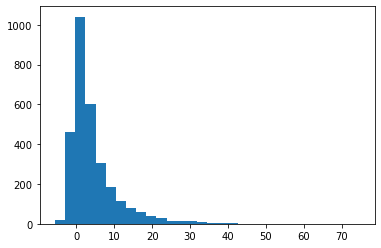
And this draws samples from the variable “d” above:
[14]:
d_sample = [d.evaluate() for _ in range(3000)]

plt.hist(d_sample, bins=30);
To generate example date for a single variable, it may sufficient to call its evaluate() method, but not very efficient. This is done better with the help of halerium models, which also allow one to perform other, more complex statistical tasks.
Static and dynamic variables#
Random variables in halerium come in the flavours Variable and StaticVariable. The difference between these comes into play when one can have multiple examples for a quantity of the modelled system with possibly different values but all drawn from the same distribution. Such random variables that follow the same distribution but can have a different value in each example should be represented by instances of Variable. In contrast, random variables that have the same value for each
example, like an internal system parameter, should be represented by instances of StaticVariable.
For example, when constructing a machine learning model, the features and targets of the model should be Variables and the trainable parameters of the model should be StaticVariables.
Entities#
Entities are containers (similar C structs) that help organize and group variables and thereby provide structure to models. Entities can contain variables as well as other entities. This means that one can create a whole hierarchy of entities.
Like variables, entities have a name. To create an entity that is contained in another entity, the contained entity has to be created within the context of the containing entity using python’s “with” clause. Similarly, variables contained in the entity need to be created within the context of the entity.
This creates an entity “car”, that contains an entity “body” and an entity “engine”, which contains variables “power” and “weight”:
[15]:
car = Entity("car")
with car:
    body = Entity("body")
    engine = Entity("engine")
    with engine:
        power = Variable("power", mean=160., variance=4.)
        weight = Variable("weight", mean=2.4, variance=0.01)
Creating entities or variables in the context of the entity makes these entities or variables “children” of the entity.
To see what direct children an the entity has we can use the children attribute of the entity:
[16]:
car.children
[16]:
{'body': <halerium.Entity at 0x210d927ef08: name='body', global_name='car/body'>,
 'engine': <halerium.Entity at 0x210d9220bc8: name='engine', global_name='car/engine'>}
There is also a function that can be used to gain a quick overview of the structure of an entitry:
[17]:
print_child_tree(car)
car
├─body
└─engine
  ├─power
  └─weight
The child of an entity is essentilly an attribute of that entity. We indeed can use python’s attribute syntax to access children. For example:
[18]:
print(car.body)
print(car.engine)
print(car.engine.power)
print(car.engine.weight)
<halerium.Entity 'car/body'>
<halerium.Entity 'car/engine'>
<halerium.Variable 'car/engine/power'>
<halerium.Variable 'car/engine/weight'>
Graphs#
A halerium Graph is another container for structuring models. Graphs share similiarities to functions in that they provide an encapsulated environment for (part of) a network of halerium variables together with well-defined inputs and outputs.
Graphs can contain variables, entities, as well as other graphs as subgraphs.
This creates a graph that takes a car and enhances its power by a factor that is intrinsic to the enhancement process:
[19]:
enhance_car_engine = Graph("enhance_car_engine")
with enhance_car_engine:
    with inputs:
        car = Entity("car")
        with car:
            Entity("body")
            Entity("engine")
            with car.engine:
                Variable("power", mean=160., variance=4.)
                Variable("weight", mean=2.4, variance=0.01)
    with outputs:
        enhanced_car = car.copy("enhanced_car")

    enhancement_factor = StaticVariable("enhancement_factor", mean=2.0, variance=0.3**2)

    enhanced_car.engine.power.mean = car.engine.power * enhancement_factor

hal.show(enhance_car_engine)
Subgraphs can be used to encapsulate subprocesses of a statistical model from other parts of the model. Graphs that are not subraphs can be used to represent a full statistical model. Such a graph can be handed to one of halerium’s model classes or factories to create a halerium model to perform computations on the model.
Graphs come with inputs and outputs as children. These can contain enitities and variables. Connections from the outside of a graph to its interior can only be done via Links to objects in the graph’s inputs and outputs.
Links#
A halerium Link is a connection between two Entity or (Static)Variable instances, the source and the target. The linked target is then essentially a reference to the source. So the values of all variables in the target will all mimic the values in the corresponding source variables.
Links are established by calling the link() function.
This creates a graph with two subgraphs, and then establishes a link between output of the first and the input of the second subgraph:
[20]:
make_enhanced_car = Graph("make_enhanced_car")
with make_enhanced_car:

    #the first subgraph creates a car:
    create_car = Graph("create_car")
    with create_car:
        with outputs:
            car = Entity("car")
            with car:
                Entity("body")
                Entity("engine")
                with car.engine:
                    Variable("power", mean=160., variance=4.)
                    Variable("weight", mean=2.4, variance=0.01)

    # the second subgraph takes a car and enhances its engine:
    enhance_car_engine = Graph("enhance_car_engine")
    with enhance_car_engine:
        with inputs:
            car = car.copy("car")
        with outputs:
            enhanced_car = car.copy("enhanced_car")

        enhancement_factor = StaticVariable("enhancement_factor", mean=2.0, variance=0.3**2)

        enhanced_car.engine.power.mean = car.engine.power * enhancement_factor

    with outputs:
        enhanced_car = car.copy("enhanced_car")

    #link the car in the outputs of the first subgraph and the car in the inputs of the second subgraph:
    link(make_enhanced_car.create_car.outputs.car, make_enhanced_car.enhance_car_engine.inputs.car)

    #link the car in the outputs of the second subgraph and the car in the outputs of the graph itself:
    link(make_enhanced_car.enhance_car_engine.outputs.enhanced_car, make_enhanced_car.outputs.enhanced_car)

hal.show(make_enhanced_car)
A primary purpose of links is to connect graphs, e.g. to chain subgraphs as the example illustrates.
There are various rules in place on what can be linked:
Linkable objects must be of type
Entityor(Static)Variable.Link source and target must be of the same type.
The source and the target must have compatible structures. In particular, for every variable in the target there must be a corresponding variable of the same shape in the source.
A link source can be:
an input (sub-)entity/variable of a graph,
an output (sub-)entity/variable of a child graph of a graph,
a free (sub-)entity/variable of a graph.
A link target can be:
an output (sub-)entity/variable of a graph,
an input (sub-)entity/variable of a child graph of a graph,
a free (sub-)entity/variable of a graph.
An entity or variable can be the source of many links, but the tarkget of at most one link.
Copying#
One can copy variable, entity, and graph instances by calling their copy method. In the example for graphs, we used copy on the entity “car” to create an entity called “enhanced_car”. The copy method takes the name of the copy as argument:
[21]:
car = Entity("car")
with car:
    Entity("body")
    Entity("engine")
    with car.engine:
        Variable("power", mean=160., variance=4.)
        Variable("weight", mean=2.4, variance=0.01)

another_car = car.copy("another_car")

print_child_tree(car)
print_child_tree(another_car)
car
├─body
└─engine
  ├─power
  └─weight
another_car
├─body
└─engine
  ├─power
  └─weight
Templates#
One can also create templates from an instance. This does not immediately create another instance, but the template can then be called to create new instances:
[22]:
car = Entity("car")
with car:
    Entity("body")
    Entity("engine")
    with car.engine:
        Variable("power", mean=160., variance=4.)
        Variable("weight", mean=2.4, variance=0.01)

car_template = car.get_template("car_template")

another_car = car_template("another_car")

yet_another_car = car_template("yet_another_car")

print_child_tree(car)
print_child_tree(another_car)
print_child_tree(yet_another_car)
car
├─body
└─engine
  ├─power
  └─weight
another_car
├─body
└─engine
  ├─power
  └─weight
yet_another_car
├─body
└─engine
  ├─power
  └─weight
Models#
Halerium graphs are the ‘blueprints’ of statistical models. They describe a statistical model, but they don’t offer functionality to evaluate them. This is what halerium models are for.
Halerium models implement a specific algorithm/solution strategy in order to do actual numerical calculations on the statistical model described by a halerium graph. Upon creation, a model instance takes a graph describing the statistical model and possibly some data to condition the model on, and combines that graph, that data, and a solving strategy to provide answers to statistical questions such as, e.g., means or variances of the model’s random variables.
Models can be instantiated directly, or by calling the factory functions get_generative_model(), get_posterior_model(), or get_optimizer_model().
Generative models#
Generative models can be used to perform simulations of statisticl models.
This creates an instance of ForwardModel:
[23]:
car_model = get_generative_model(graph=make_enhanced_car,
                                 data=DataLinker(n_data=1000)
                                )

car_model
[23]:
<halerium.core.model.forward_model.ForwardModel at 0x210d91c75c8>
This model is purely for generating data in a feed-forward fashion. Information from data only flows forwards along the dependencies of the structure.
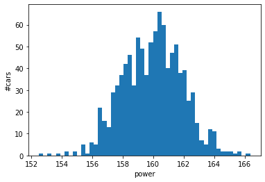
The model can be used, e.g., to generate examples:
[24]:
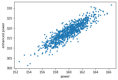
power_sample, enhanced_power_sample = car_model.get_example((
    make_enhanced_car.create_car.outputs.car.engine.power,
    make_enhanced_car.outputs.enhanced_car.engine.power,
))

plt.hist(power_sample, bins=50);
plt.xlabel("power");
plt.ylabel("#cars");
plt.show();

plt.plot(power_sample, enhanced_power_sample, '.');
plt.xlabel("power");
plt.ylabel("enhanced power");
plt.show();
If one requires a model to also take into account the backward and sideways flow of information from data, one of the posterior model classes should be taken instead.
Posterior models#
Posterior models can be used for statistical inference and machine learning (see, e.g., more on training models and regression).
Calling get_posterior_model() returns an instance of one of halerium’s posterior model classes. These models calculate estimates for model variables taking all data and all possible directions of information flow into account.
The model classes differ in their solving strategy. Each strategy has particular advantages and drawbacks regarding speed, accuracy, and the kinds of statistical models it can solve efficiently. Which model class (and therefore solving strategy) is returned can be controlled by keyword argument ‘method’:
‘MAP’ yields a
MAPModel, which implements a gradient-based maximum posterior finder. This is usually the fastest among the models, and an adequate choice for many best-fit and machine learning tasks. It however cannot quantify the statistical spread (variance) of random variables.‘MAPFisher’ yields a
MAPFisherModel, which implements another gradient-based maximum posterior finder that can also quantifies the spread of random variables by estimating the Fisher matrix. This is the default.‘MGVI’ yields an
MGVIModel, which implements Metric Gaussian Variational Inference.‘ADVI’ yields an
ADVIModel, which implements Automatic Differentiation Variational Inference.‘MCMC’ yields and
MCMCModel, which implements a Markov chain Monte Carlo sampling algorithm. This model may be slower than the others, but given enough time, the most accurate.
For a simple example, assume, we have collected data on the power of a series of enhanced engines from our car making process:
[25]:
enhanced_power_data = [420, 410, 415, 380, 440, 460]
To provide this data to the posterior model, we can use a dictionary with the data as value and the variable that data is for as key:
[26]:
car_model = get_posterior_model(graph=make_enhanced_car,
                                 data={make_enhanced_car.enhance_car_engine.outputs.enhanced_car.engine.power: enhanced_power_data}
                                )
We can ask the posterior model to estimate the posterior mean of the enhancement factor:
[27]:
mean_enhancement_factor = car_model.get_means(make_enhanced_car.enhance_car_engine.enhancement_factor)
stddev_enhancement_factor = car_model.get_standard_deviations(make_enhanced_car.enhance_car_engine.enhancement_factor)


print(f"posterior estimate for enhancement factor = {mean_enhancement_factor} +/- {stddev_enhancement_factor}")
posterior estimate for enhancement factor = 2.6367891524615614 +/- 0.012165074100338357
This is significantly above the prior mean of 2, which is what one should expect given the above-average values for the enhanced power.
A more comprehensive discussion on using posterior models can be found in the inheritance example notebook.
Posterior models
Optimizer models#
Optimizer models can be used for optimization tasks.
get_optimizer_model() will return an instance of ForwardOptimizerModel. This model is used to calculate the optimal values for a set of variables that minimize a cost function that depends on a set of (different) variables in the graph.
Assume, the optimal output power is given by:
[28]:
optimal_output_power = 550
Let us try to tune the model to the optimal output power by tuning the enhancement factor in the interval \([0.5, 6]\) starting at a value of 2:
[29]:
def cost_function(graph):
    return (graph.outputs.enhanced_car.engine.power - optimal_output_power)**2

car_model = get_optimizer_model(
    graph=make_enhanced_car,
    adjustables = {make_enhanced_car.enhance_car_engine.enhancement_factor: [3, 0.5, 6]},
    cost_function=cost_function,
    solver="L-BFGS"
)

optimal_enhancement_factor = float(car_model.adjustables[make_enhanced_car.enhance_car_engine.enhancement_factor][0])
print(f"optimal enhancement factor = {optimal_enhancement_factor}")

output_power = car_model.get_means(make_enhanced_car.outputs.enhanced_car.engine.power)
print(f"resulting power = {output_power[0]}")
optimal enhancement factor = 3.440362845168096
resulting power = 550.8090952252322
[ ]: