Example: Inheritance and body heights

Halerium models consist of Variables, Entities and Graphs. They are the essential building blocks to create arbitrarily hierarchical models.

We want to illustrate how this works by implementing a simple inheritance model, in which we look at the dependencies between the height of parents and the height of children.

We start by importing required packages:

import warnings; warnings.simplefilter('ignore')
import halerium.core as hal
from plots import *

Let us create our first entity, a person:

person = hal.Entity("person")
with person:
    hal.Variable("height", shape=[])
    hal.Variable("genetic_factor", shape=[], mean=0, variance=75)

Now we have an Entity instance called person. In our simple world a person is fully defined by its genetic and actual height.

We can create a Template from this instance for future usage.

Person = person.get_template()

Now let’s get more specific and create a man and a woman:

man = Person("man")
with man:
    height.mean = 175 + genetic_factor
    height.variance = 25.

woman = Person("woman")
with woman:
    height.mean = 167 + genetic_factor
    height.variance = 25.

Man = man.get_template()
Woman = woman.get_template()

OK, so what happened? We defined both man and woman as a person, but then we modified each of them in a different way. Essentially we are saying, the typical man is 175cm tall and the typical woman 167cm tall. However, the actual height is modified by genetic factors of this particular person as well as a random noise around the genetic predisposition.

We also created templates of man and woman.

Now, let’s define a Graph in which a man and a woman get a daughter.

make_daughter = hal.Graph("make_daughter")
with make_daughter:
    with inputs:
        Man("father")
        Woman("mother")
    with outputs:
        Woman("daughter")
    outputs.daughter.genetic_factor.mean = (inputs.father.genetic_factor + inputs.mother.genetic_factor) / 2.
    outputs.daughter.genetic_factor.variance = 37.5

MakeDaughter = make_daughter.get_template()

So what we specified is the following: the Graph make_daughter has two inputs: mother and father. mother is an instace of Woman, father is an instance of Man. The output is a daughter, an instance of Woman.

If we left it at that there would have been no dependence of the daughter height on her parents. We specified this dependency in the the two last lines of code. We specified that the genetic_height of the daughter fluctuates around the mean genetic height of her parents (a super simple model of combination and mutation).

Now let’s repeat that for a son:

make_son = hal.Graph("make_son")
with make_son:
    with inputs:
        Man("father")
        Woman("mother")
    with outputs:
        Man("son")
    outputs.son.genetic_factor.mean = (inputs.father.genetic_factor + inputs.mother.genetic_factor) / 2.
    outputs.son.genetic_factor.variance = 37.5

MakeSon = make_son.get_template()

Now we can create the Graph for a full family.

Let’s call the parents alice and bob

family = hal.Graph("family")
with family:
    Woman("alice")
    Man("bob")

alice and bob are happy together so let’s make two children, harry and sally

with family:
    MakeSon("make_harry")
    MakeDaughter("make_sally")

However, we have not specified yet, that alice and bob are actually the parents of both of them. We can do that by linking:

with family:
    hal.link(alice, make_harry.inputs.mother)
    hal.link(alice, make_sally.inputs.mother)
    hal.link(bob, make_harry.inputs.father)
    hal.link(bob, make_sally.inputs.father)

Now we specified that the father in make_harry was actually bob and not somebody else.

We can inspect the family graph in the interactive GUI

hal.show(family)

Now we are done and can start to generate random family examples:

We start by creating a generative model.

gen_model = hal.get_generative_model(family)

The generative model is the simplest kind of model, that allows us to create artificial data and/or do forward simulations. For example we can get example samples:

sample = gen_model.get_samples({"alice": family.alice.height,
                                 "bob": family.bob.height,
                                 "harry": family.make_harry.outputs.son.height,
                                 "sally": family.make_sally.outputs.daughter.height,})

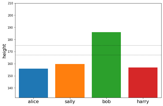
plot_family_heights(sample)
sample

{'alice': [array([155.97561197])],
 'bob': [array([185.9337903])],
 'harry': [array([156.81862308])],
 'sally': [array([159.64632049])]}

Or the mean values of specific variables in our graph

means = gen_model.get_means({"alice": family.alice.height,
                             "bob": family.bob.height,
                             "harry": family.make_harry.outputs.son.height,
                             "sally": family.make_sally.outputs.daughter.height,}, n_samples=1000)
means

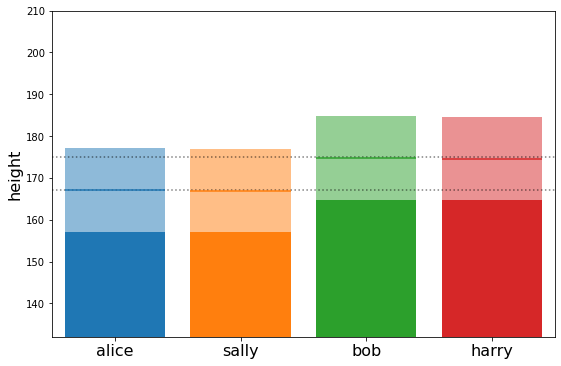
{'alice': array([167.0568489]),
 'bob': array([174.79392627]),
 'harry': array([174.60622365]),
 'sally': array([166.89633946])}

or the standard_deviations …

stds = gen_model.get_standard_deviations({"alice": family.alice.height,
                                          "bob": family.bob.height,
                                          "harry": family.make_harry.outputs.son.height,
                                          "sally": family.make_sally.outputs.daughter.height,}, n_samples=1000)

plot_family_heights(means, stds)
stds

{'alice': array([10.06116075]),
 'bob': array([9.96899764]),
 'harry': array([9.94216823]),
 'sally': array([9.92119949])}

Now let’s simulate how the family of Alice and Bob would develop if we actually knew both their genetic factor and their height

Let’s say Alice has a genetic_factor of +5, but still was of average height: 167cm.

Bob has a genetic_factor of +5 as well, but is of average height, too: 175cm

I guess they did not eat their spinach.

alice_gen_factor = 5.
alice_height = 167.
bob_gen_factor = 5
bob_height = 175.

family.alice.genetic_factor

<halerium.Variable at 0x21b43670208: name='genetic_factor', shape=(), global_name='family/alice/genetic_factor', dynamic=True, distribution=NormalDistribution>

Now lets create a generative model conditioned to these data

gen_model_wdata = hal.get_generative_model(family, data={family.alice.genetic_factor: alice_gen_factor,
                                                         family.alice.height: alice_height,
                                                         family.bob.genetic_factor: bob_gen_factor,
                                                         family.bob.height: bob_height})

cond_means = gen_model_wdata.get_means({"alice": family.alice.height,
                                        "bob": family.bob.height,
                                        "harry": family.make_harry.outputs.son.height,
                                        "sally": family.make_sally.outputs.daughter.height,}, n_samples=1000)
cond_means

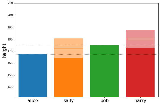
{'alice': array([167.]),
 'bob': array([175.]),
 'harry': array([180.02715988]),
 'sally': array([172.43563186])}

cond_stds = gen_model_wdata.get_standard_deviations({"alice": family.alice.height,
                                                     "bob": family.bob.height,
                                                     "harry": family.make_harry.outputs.son.height,
                                                     "sally": family.make_sally.outputs.daughter.height,}, n_samples=1000)
cond_stds

{'alice': array([0.]),
 'bob': array([0.]),
 'harry': array([7.5037483]),
 'sally': array([7.95827691])}

plot_family_heights(cond_means, cond_stds)

Now what has changed? We see that alice’s and bob’s height are fixed to the linked data. Their children are taller than both of them, since we gave both alice and bob positive genetic factors.

The standard deviation of of the heights of harry and sally was reduced, too. Since we now added information about their parents.

OK, now let’s make this a little bit more interesting

In reality we would not know the genetic_factor of both alice and bob, but just their heights. This time lets make alice and bob taller than average:

post_model = hal.get_posterior_model(family, data={family.alice.height: 172,
                                                   family.bob.height: 180})

This time we used a posterior model. This model can solve any dependency, be it forward, backward or other.

post_means = post_model.get_means({"alice": family.alice.height,
                                   "bob": family.bob.height,
                                   "harry": family.make_harry.outputs.son.height,
                                   "sally": family.make_sally.outputs.daughter.height,}, n_samples=100)
post_means

{'alice': array([172.]),
 'bob': array([180.]),
 'harry': array([178.75055174]),
 'sally': array([170.74982655])}

post_stds = post_model.get_standard_deviations({"alice": family.alice.height,
                                                "bob": family.bob.height,
                                                "harry": family.make_harry.outputs.son.height,
                                                "sally": family.make_sally.outputs.daughter.height,}, n_samples=100)
post_stds

{'alice': array([0.]),
 'bob': array([0.]),
 'harry': array([8.89468819]),
 'sally': array([8.36109147])}

plot_family_heights(post_means, post_stds)

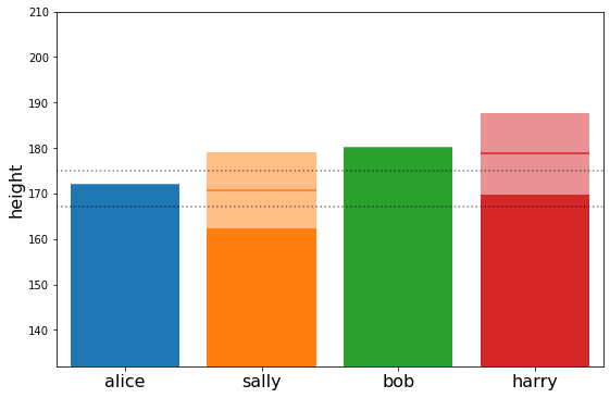
Interesting… we see that the expected height of harry and sally is taller that average but not quite as tall as their parents. This effect is known as ‘regression to the mean’. We can understand it better by looking at the estimated genetic_factors of alice and bob.

post_model.get_means({"alice genfactor": family.alice.genetic_factor,
                      "bob genfactor": family.bob.genetic_factor,}, n_samples=100)

{'alice genfactor': array([3.75000001]), 'bob genfactor': array([3.75000001])}

Both alice and bob were 5cm taller than the average man or woman. As we can see, 3/4 of this extra height were estimated into the genetic_factor. The rest was explained as a random fluctuation of the height of alice and bob around their genetic predisposition.

This is because the variance of the genetic factor was exactly 3 times greater that the variance of the actual height around its genetic predisposition (75 vs 25).

Consequently, the genetic factor of their children is

post_model.get_means({"harry genfactor": family.make_harry.outputs.son.genetic_factor,
                      "sally genfactor": family.make_sally.outputs.daughter.genetic_factor,}, n_samples=100)

{'harry genfactor': array([3.75030801]),
 'sally genfactor': array([3.74999697])}

And since for them the changes of being taller or shorter than their genetic predisposition are equal, their average tends exactly to their genetic predisposition.

Now lets turn this around. What does the height of the children tell me about the height of the parents.

post_model2 = hal.get_posterior_model(family, data={family.make_harry.outputs.son.height: 180,
                                                    family.make_sally.outputs.daughter.height: 172})

post_means2 = post_model2.get_means({"alice": family.alice.height,
                                     "bob": family.bob.height,
                                     "harry": family.make_harry.outputs.son.height,
                                     "sally": family.make_sally.outputs.daughter.height,}, n_samples=100)
post_stds2 = post_model2.get_standard_deviations({"alice": family.alice.height,
                                                  "bob": family.bob.height,
                                                  "harry": family.make_harry.outputs.son.height,
                                                  "sally": family.make_sally.outputs.daughter.height,}, n_samples=100)
plot_family_heights(post_means2, post_stds2)
post_means2

{'alice': array([169.72737024]),
 'bob': array([177.72675745]),
 'harry': array([180.]),
 'sally': array([172.])}

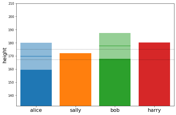
We see the regression to the mean also works backwards.