Creating MA, AR, and ARMA Graphs

import numpy as np
import matplotlib.pyplot as plt

import halerium.core as hal

By using this Application, You are agreeing to be bound by the terms and conditions of the Halerium End-User License Agreement that can be downloaded here: https://erium.de/halerium-eula.txt

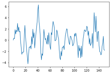
the MA model (moving average)

An MA model is defined as

\[\begin{split}y_t = c + \epsilon_t + \sum_{j=1}^q b_j \epsilon_{t-j}\\ \epsilon_t \hookleftarrow N(\epsilon_t| 0, \sigma^2)\end{split}\]

we can create this explicitly in Halerium using the TimeIndex.

q = 5
sigma = 1.
sigma_obs = 1.e-2

ma_graph = hal.Graph("graph")
with ma_graph:
    hal.StaticVariable("b", shape=(q,), mean=0, variance=1)
    hal.StaticVariable("c", shape=(), mean=0, variance=1)

    hal.Variable("epsilon", mean=0, variance=sigma**2)
    hal.Variable("y")
    y.mean = sum([
        b[i] * epsilon[hal.TimeIndex-i-1]
        for i in range(q)
    ]) + c
    y.variance = (sigma/100)**2
    # TODO: or the next
    hal.Variable("observed", mean=y, variance=sigma_obs**2)
    # this "observed" variable is strictly speaking not part of the model,
    # but it is recommended when we want to fit data to the model as it allows us
    # to include observation noise.

The [TimeIndex...] is a shorthand convenience for the TimeShift operator with initial values set to 0.

So instead of epsilon[TimeIndex-i-1] we could write TimeShift(epsilon, shift=-i-1, initial_values=0).

Note that in the Graph definition we did no specify the length of the time series. Halerium will utilize the dynamic axis of the Variable class for the time steps, which means we specify the length of the time series with n_data.

data = hal.get_data_linker(
    {ma_graph.b: np.ones(q),
     ma_graph.c: 0.},
    n_data=150
)
m = hal.get_generative_model(ma_graph, data)
plt.plot(m.get_example(ma_graph.y))

[<matplotlib.lines.Line2D at 0x193ad6fc940>]

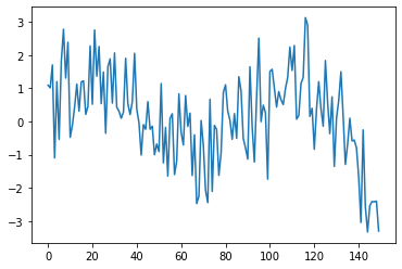
the AR model (autoregressive)

An AR model is defined as

\[y_t = c + \epsilon_t + \sum_{i=1}^p a_i y_{t-i}\]

which as an Halerium graph is

p = 7
sigma = 1.
sigma_obs = 1.e-2

ar_graph = hal.Graph("graph")
with ar_graph:
    hal.StaticVariable("a", shape=(p,), mean=0, variance=1)
    hal.StaticVariable("c", shape=(), mean=0, variance=1)

    hal.Variable("y")
    y.mean = sum([
        a[i] * y[hal.TimeIndex-i-1]
        for i in range(p)
    ]) + c
    y.variance = sigma**2 # since there is no moving average in the AR model
                          # time we include epsilon as the variance of y.

    hal.Variable("observed", mean=y, variance=sigma_obs**2)
    # this "observed" variable is strictly speaking not part of the model,
    # but it is recommended when we want to fit data to the model as it allows us
    # to include observation noise.

Let’s look at an example for the AR process

data = hal.get_data_linker(
    {ar_graph.a: np.ones(p)/p,
     ar_graph.c: 0.},
    n_data=150
)
m = hal.get_generative_model(ar_graph, data)
plt.plot(m.get_example(ar_graph.y))

[<matplotlib.lines.Line2D at 0x193ae10e160>]

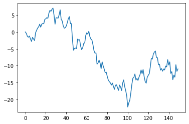
the ARMA model

The ARMA model combines the autoregressive and moving average concept

\[y_t = c + \epsilon_t + \sum_{i=1}^p a_i y_{t-i} + \sum_{j=1}^q b_j \epsilon_{t-j}\]

p = 7
q = 5
sigma = 1.
sigma_obs = 1.e-2

arma_graph = hal.Graph("graph")
with arma_graph:
    hal.StaticVariable("a", shape=(p,), mean=0, variance=1)
    hal.StaticVariable("b", shape=(q,), mean=0, variance=1)
    hal.StaticVariable("c", shape=(), mean=0, variance=1)

    hal.Variable("epsilon", mean=0, variance=sigma**2)

    hal.Variable("y")

    ar_contrib = sum([
        a[i] * y[hal.TimeIndex-i-1]
        for i in range(p)
    ])

    ma_contrib = sum([
        b[i] * epsilon[hal.TimeIndex-i-1]
        for i in range(q)
    ])

    y.mean = c + ar_contrib + ma_contrib
    y.variance = (sigma/100)**2
    # OR
    hal.Variable("observed", mean=y, variance=sigma_obs**2)
    # this "observed" variable is strictly speaking not part of the model,
    # but it is recommended when we want to fit data to the model as it allows us
    # to include observation noise.

data = hal.get_data_linker(
    {arma_graph.a: np.ones(p)/p,
     arma_graph.b: np.ones(q),
     arma_graph.c: 0.},
    n_data=150
)
m = hal.get_generative_model(arma_graph, data)
plt.plot(m.get_example(arma_graph.y))

[<matplotlib.lines.Line2D at 0x193ae18df40>]

the ARIMA model

The arima model is an integrated ARMA model. So the ARMA process is simply intergrated \(d\) times.

In Halerium it can be defined like this

d = 3
p = 7
q = 5
sigma = 1.
sigma_obs = 1.e-2

arima_graph = hal.Graph("graph")
with arima_graph:
    hal.StaticVariable("a", shape=(p,), mean=0, variance=1)
    hal.StaticVariable("b", shape=(q,), mean=0, variance=1)
    hal.StaticVariable("c", shape=(), mean=0, variance=1)

    hal.Variable("epsilon", mean=0, variance=sigma**2)

    hal.Variable("x")

    ar_contrib = sum([
        a[i] * x[hal.TimeIndex-i-1]
        for i in range(p)
    ])

    ma_contrib = sum([
        b[i] * epsilon[hal.TimeIndex-i-1]
        for i in range(q)
    ])

    x.mean = c + ar_contrib + ma_contrib

    # x follows the ARMA model

    # to integrate we define a helper variable int_i
    temp = x
    for i in range(d):
        temp_integrator = hal.Variable(f"int_{i}")
        temp_integrator.mean = temp_integrator[hal.TimeIndex-1] + temp
        temp = temp_integrator

    hal.Variable("y")
    y.mean = temp

    hal.Variable("observed", mean=y, variance=sigma_obs**2)
    # this "observed" variable is strictly speaking not part of the model,
    # but it is recommended when we want to fit data to the model as it allows us
    # to include observation noise.

data = hal.get_data_linker(
    {arma_graph.a: np.ones(p)/p,
     arma_graph.b: np.ones(q),
     arma_graph.c: 0.},
    n_data=150
)
m = hal.get_generative_model(arima_graph, data)
x_ex, y_ex = m.get_example([arima_graph.x, arima_graph.y])

plt.plot(y_ex)

[<matplotlib.lines.Line2D at 0x193adf84160>]

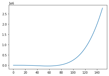
Note that an ARIMA model is not stationary, but can show significant growth and trends due to the integration. It is therefore often used to fit non-stationary time-series. In practice one usually differentiates the data and uses an ARMA model on the differetiated data though.