Gaussian Process Regression

The standard regression functionality approximates the functional relation between input variables and output variables by a linear or low-order polynomial. This can be an over-simplification at times.

A more general approach is to approximate the functional relationship as the superposition of one-dimensional Gaussian processes. Gaussian processes are auto-correlated (and therefore smooth) along a spatial axis.

Background: The Principles of Gaussian Processes

Let us first understand what Gaussian processes in halerium can be constructed and what it looks like.

Imports

We will need numpy and halerium for constructing the Gaussian process and pylab for plotting.

import numpy as np
import halerium.core as hal
import pylab as pl

We now construct a Gaussian process

g = hal.Graph("g")
with g:
    hal.StaticVariable("uncorrelated_source", shape=(100,),
                       mean=0, variance=1)
    kernel = np.exp(-0.5*np.arange(-20, 21)**2 / 5**2) / 2
    hal.StaticVariable("gaussian_process", shape=(100,),
                       mean=hal.math.convolve(uncorrelated_source, kernel))

Here we have constructed an uncorrelated source field. On this field the correlation structure is imposed by convolving it with a kernel. Let’s have a look at some examples.

# the evaluate function allows us to conveniently get a generative example
gaussian_process_examples = [g.gaussian_process.evaluate() for i in range(3)]
pl.figure(figsize=(12, 7))
[pl.plot(gp_ex) for gp_ex in gaussian_process_examples]

[[<matplotlib.lines.Line2D at 0x1ba9de2a808>],
 [<matplotlib.lines.Line2D at 0x1ba9dbc0088>],
 [<matplotlib.lines.Line2D at 0x1ba9de36f48>]]

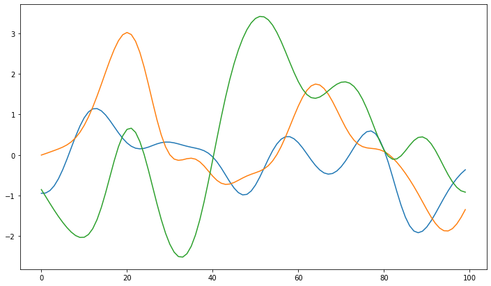
As we can see gaussian processes can be interpreted smooth functions. Due to the kernel the process has a preferred fluctuation scale and tends to go back to the origin at zero. We will see how this changes once we introduce data.

Using a Gaussian process as a function

To use a Gaussian process as a function we have to be able to evaluate it at arbitrary positions. We can do this using iterpolation.

g = hal.Graph("g")
with g:
    hal.StaticVariable("uncorrelated_source", shape=(100,),
                       mean=0, variance=1)
    kernel = np.exp(-0.5*np.arange(-20, 21)**2 / 5**2)
    hal.StaticVariable("gaussian_process", shape=(100,),
                       mean=hal.math.convolve(uncorrelated_source, kernel))

    hal.Variable("x", mean=0, variance=1)
    evaluated = hal.math.interpolate(
        evaluation_points=x, # where the interpolation is evaluated
        support_point_values=gaussian_process,
        support_point_base=-3, # we want the 100 points of the gaussian process
        support_point_spacing=6/100 # to cover the interval [-3, 3]
    )
    hal.Variable("y", mean=evaluated, variance=0.01)

Now the graph uses the gaussian process as a function that relates x and y as y=f(x).

x_value_example = np.linspace(-5, 5, 1000)
generative_model = hal.get_generative_model(g, data={g.x: x_value_example})
y_value_example = generative_model.get_example(g.y)
pl.figure(figsize=(12, 7))
pl.plot(x_value_example, y_value_example)

[<matplotlib.lines.Line2D at 0x1baa3bdc8c8>]

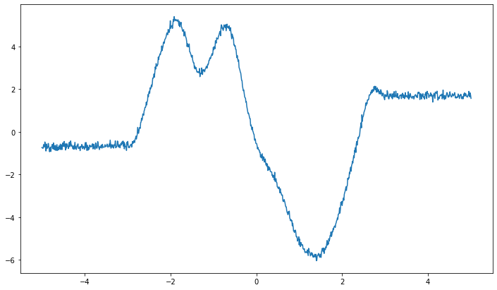
We can see two things here: 1. the function is noisy due to the variance of the variable y 2. outside of the interpolation interval [-3, 3] the function becomes constant (apart from the noise)

Learning a Gaussian process from data

Create training data

Let us now create training data from which we hope to learn the Gaussian process.

np.random.seed(151)
x_data = np.random.randn(100)
# we remove the interval [0.0, 1.0] for demonstration purposes
x_data = x_data[(x_data < 0.) | (x_data > 1.0)]

def real_function(x):
    return np.sin(4*np.tanh(x/1.5))

y_data = real_function(x_data) + np.random.randn(*x_data.shape)*0.1

pl.figure(figsize=(12, 7))
pl.scatter(x_data, y_data, label="data", color="b", marker="x")
pl.plot(np.linspace(-4, 4, 1000),
        real_function(np.linspace(-4, 4, 1000)),
        label="real function", color="k")
pl.legend()

<matplotlib.legend.Legend at 0x1baa3c54b48>

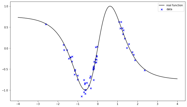
Our training data are a noisy representation of the real function with a gap in the interval [0, 1].

Train

We can now use these data to infer the most likely Gaussian process representation.

posterior_model = hal.get_posterior_model(g,
                                          data={g.x: x_data,
                                                g.y: y_data})
trained_graph = posterior_model.get_posterior_graph()

Now we have a trained graph in which the posterior probability of the gaussian process is encoded. We can use this trained graph to make a prediction on a test set

x_test = np.linspace(-4, 4, 1000)
prediction_model = hal.get_generative_model(trained_graph, data={g.x: x_test})
y_pred_mean = prediction_model.get_means(g.y, n_samples=1000)
y_pred_std = prediction_model.get_standard_deviations(g.y, n_samples=1000)

pl.figure(figsize=(12, 7))
pl.plot(x_test, real_function(x_test), color="k", label="real function")
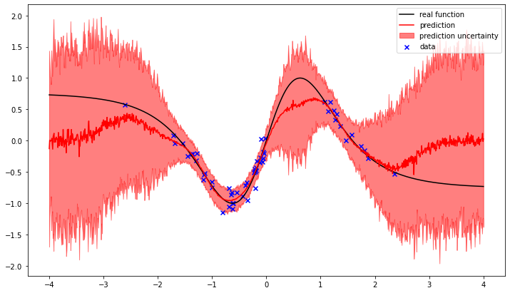
pl.plot(x_test, y_pred_mean, color="r", label="prediction")
pl.fill_between(x_test, y_pred_mean-y_pred_std, y_pred_mean+y_pred_std,
                color="r", alpha=0.5, label="prediction uncertainty")
pl.scatter(x_data, y_data, label="data", color="b", marker="x")
pl.legend()

<matplotlib.legend.Legend at 0x1baa78f48c8>

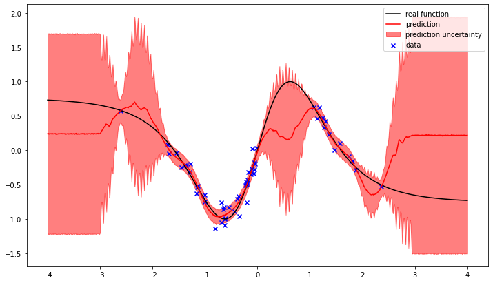
We can see how the gaussian process attempts to interpolate between the observed data points. The training result is the most likely balance between the prior correlation structure of the gaussian process and the noise likelyhood of the observed data.

In the regions without observations the difference between the prediction and the real function increases, as does the uncertainty.

This is the way Gaussian process regression works.

Gaussian process using convenience functions

Halerium offers the user a convenience function that constructs an appropriate Gaussian process regression between variables with a single command.

g2 = hal.Graph("g")
with g2:
    hal.Variable("x", mean=0, variance=1)
    hal.Variable("y")
    hal.regression.connect_via_gaussian_process(
        name_prefix="regression",
        inputs=x,
        outputs=y,
        connect_outputs_scale_parameter=True, # this means we learn the variance as well
    )

The connect_via_gaussian_process created all the necessary variables and operations for a gaussian process regression. Training and evaluation works the same way as above, but this time we use the Trainer and Predictor for convenience.

trained_graph2 = hal.model.Trainer(g2, data={g2.x: x_data, g2.y: y_data}, method="MGVI")()

y_pred_mean2, y_pred_std2 = hal.Predictor(
    trained_graph2, data={g2.x: x_test}, measure=("mean", "std"))(g2.y)

pl.figure(figsize=(12, 7))
pl.plot(x_test, real_function(x_test), color="k", label="real function")
pl.plot(x_test, y_pred_mean2, color="r", label="prediction")
pl.fill_between(x_test, y_pred_mean2-y_pred_std2, y_pred_mean2+y_pred_std2,
                color="r", alpha=0.5, label="prediction uncertainty")
pl.scatter(x_data, y_data, label="data", color="b", marker="x")
pl.legend()

<matplotlib.legend.Legend at 0x1baac93f1c8>

The reconstruction is slightly different, because the connect_via_gaussian_process function uses a slightly different kernel. Additionally the variance of y is also learned, whereas in the example above it was known.

Multiple or multivariate regression inputs and outputs

The Gaussian process serves us as a representation of a 1-dimensional function, i.e. a function \(f: \mathbb{R} \rightarrow \mathbb{R}\).

To represent functions \(f: \mathbb{R}^N \rightarrow \mathbb{R}^M\) the following simplification is applied:

\[\left(f(x)\right)_i = \sum_j h_{ij}(x_j).\]

Here \(h_{ij}\) is a 1-dimensional function \(f: \mathbb{R} \rightarrow \mathbb{R}\). This means the function is constructed separately for each output entry by summing independent 1-dimensional functions applied to each input entry.

Let us see how this works in practice.

We construct a Graph with multiple multivariate variables and connect them.

graph = hal.Graph("graph")
with graph:
    # a is a 4-dimensional vector with different means and standard deviations for its entries
    hal.Variable("a", shape=(4,), mean=-np.arange(1, 5), variance=np.arange(1, 5))
    # b is a 2x3-dimensional matrix
    hal.Variable("b", shape=(2, 3), mean=0, variance=0.001)

    # c is a 2x2-dimensional matrix
    hal.Variable("c", shape=(2, 2), variance=0.1)
    # d is a scalar
    hal.Variable("d", variance=0.1)

    hal.regression.connect_via_gaussian_process(
        name_prefix="regression",
        inputs=[a, b],
        outputs=[c, d],
        # For the regression to work properly it needs to know
        # the locations and scales of the inputs and outputs.
        # Alternatively you can standardize your data.
        inputs_location=[-np.arange(1, 5), 0],
        inputs_scale=[np.sqrt(np.arange(1, 5)), np.sqrt(0.001)],
        # we just define these here, normally they would come from your data
        outputs_location=[5., 5.],
        outputs_scale=[10., 10.],
        # we do not want to fit the variances here
        connect_outputs_scale_parameter=False,
    )

Now we create an example with 200 data points

data_a, data_b, data_c, data_d = hal.get_generative_model(
    graph, data=hal.get_data_linker(n_data=200)).get_example(
    [graph.a, graph.b, graph.c, graph.d])

and split them into training and test data.

train_data_a = data_a[:150]
train_data_b = data_b[:150]
train_data_c = data_c[:150]
train_data_d = data_d[:150]

test_data_a = data_a[150:]
test_data_b = data_b[150:]
test_data_c = data_c[150:]
test_data_d = data_d[150:]

Now we train the graph (this will take ~1 minute)…

train_data = {
    graph.a: train_data_a,
    graph.b: train_data_b,
    graph.c: train_data_c,
    graph.d: train_data_d
}

import time
t_start = time.time()
model = hal.get_posterior_model(graph, train_data)
tr_graph = model.get_posterior_graph()
print(time.time() - t_start)

41.167240858078

…and check whether we can predict the test set.

test_data = {
    graph.a: test_data_a,
    graph.b: test_data_b
}

pr_model = hal.get_generative_model(tr_graph, test_data)
pred_c_mean, pred_d_mean = pr_model.get_means([graph.c, graph.d])
pred_c_std, pred_d_std = pr_model.get_standard_deviations([graph.c, graph.d])

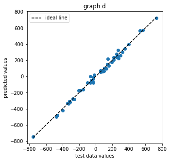
pl.figure(figsize=(5,5))
pl.scatter(test_data_d, pred_d_mean)
pl.xlabel("test data values")
pl.ylabel("predicted values")
pl.title("graph.d")
pl.plot([test_data_d.min(), test_data_d.max()],
        [test_data_d.min(), test_data_d.max()],
        color="k", ls="--", label="ideal line")
pl.legend()

<matplotlib.legend.Legend at 0x1baac820cc8>

pl.figure(figsize=(10,10))
for i, j in [[0,0], [0,1], [1,0], [1,1]]:
    ax = pl.subplot(2,2,2*i+j+1)
    ax.scatter(test_data_c[:, i, j], pred_c_mean[:, i, j])
    ax.set_xlabel("test data values")
    ax.set_ylabel("predicted values")
    ax.set_title(f"graph.c[{i},{j}]")
    ax.plot([test_data_c[:,i,j].min(), test_data_c[:,i,j].max()],
            [test_data_c[:,i,j].min(), test_data_c[:,i,j].max()],
            color="k", ls="--", label="ideal line")
    ax.legend()

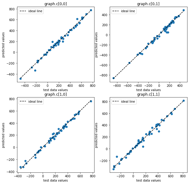
We can see that the trained graph yields accurate predictions.

More on connect_via_gaussian_process

Let’s go through the arguments of connect_via_gaussian_process.

gg = hal.Graph("gg")
with gg:
    hal.Variable("x", mean=0, variance=1)
    hal.Variable("y")
    hal.regression.connect_via_gaussian_process(
        name_prefix="regression",
        inputs=x,
        outputs=y,
        connect_outputs_scale_parameter=True,
        inputs_location=0,
        inputs_scale=1,
        outputs_location=0,
        outputs_scale=1,
        interpolation_points=100,
        interpolation_range=4.,
        kernel_correlation_length=0.4,
        kernel_size=21
    )

The first argument name_prefix is used to name the entities in the graph holding the regression parameters:

from halerium.core.utilities.print import print_child_tree
print_child_tree(gg)

gg
├─regression_y
│ ├─location
│ │ ├─source_field
│ │ └─field
│ └─log_scale
│   ├─source_field
│   └─field
├─inputs
├─outputs
├─x
└─y

Printing the graph’s children reveals that besides regression parameters for the mean of y in regression_y.location, there are also regression parameters for the variance of y in regression_y.log_scale. Thus, the mean of y as well as the residual scatter of y is learned as a Gaussian process of x.

The argument inputs specifies the input variables for the regression. This can be either a single variable or a list of variables.

The argument outputs specifies the output variables of the regression, either as a single variable, or a list of variables.

The argument connect_outputs_scale_parameter specifies whether to learn the variance(s) as field(s) as well. With False the printout of the graphs children would not have contained the log_scale entity.

The arguments inputs_location=0, inputs_scale=1, outputs_location=0, and outputs_scale=1 allow one to directly include scaling of the data for standardization in the regression. Standardization of the data would otherwise be a required step of data preparation. Here, one just needs to provide the empirical location and scale parameters of the data.

The argument interpolation_points specifies the amount of points in each 1-D Gaussian random field. With more points finer functional details can be captured, but computation time is increased.

The argument interpolation_range specifies the interpolation range in units of the inputs_scale. The interpolation range is [inputs_location-interpolation_range*inputs_scale, inputs_location+interpolation_range*inputs_scale].

The argument kernel_correlation_length defines the correlation length imposed by the kernel. It too is given w.r.t to the inputs scales.

The argument kernel_size defines the kernels size. A larger kernel imposes the correlation structure more exactly, but requires more computational effort.

More on these and a number of further arguments can be found in the documentation for connect_via_gaussian_process.