Causal Structures - applied on the California School data set#
The imports
[1]:
import numpy as np
import pydataset
import pylab as pl

from halerium import CausalStructure
from halerium import Evaluator
The California Test Score Data Set#
In this example we apply the CausalStructure class to the California Test Score Data Set. The preferred data format to use with CausalStructure is the pandas DataFrame.
[2]:
data = pydataset.data("Caschool")
data
[2]:
| distcod | county | district | grspan | enrltot | teachers | calwpct | mealpct | computer | testscr | compstu | expnstu | str | avginc | elpct | readscr | mathscr | |
|---|---|---|---|---|---|---|---|---|---|---|---|---|---|---|---|---|---|
| 1 | 75119 | Alameda | Sunol Glen Unified | KK-08 | 195 | 10.900000 | 0.510200 | 2.040800 | 67 | 690.799988 | 0.343590 | 6384.911133 | 17.889910 | 22.690001 | 0.000000 | 691.599976 | 690.000000 |
| 2 | 61499 | Butte | Manzanita Elementary | KK-08 | 240 | 11.150000 | 15.416700 | 47.916698 | 101 | 661.200012 | 0.420833 | 5099.380859 | 21.524664 | 9.824000 | 4.583333 | 660.500000 | 661.900024 |
| 3 | 61549 | Butte | Thermalito Union Elementary | KK-08 | 1550 | 82.900002 | 55.032299 | 76.322601 | 169 | 643.599976 | 0.109032 | 5501.954590 | 18.697226 | 8.978000 | 30.000002 | 636.299988 | 650.900024 |
| 4 | 61457 | Butte | Golden Feather Union Elementary | KK-08 | 243 | 14.000000 | 36.475399 | 77.049202 | 85 | 647.700012 | 0.349794 | 7101.831055 | 17.357143 | 8.978000 | 0.000000 | 651.900024 | 643.500000 |
| 5 | 61523 | Butte | Palermo Union Elementary | KK-08 | 1335 | 71.500000 | 33.108601 | 78.427002 | 171 | 640.849976 | 0.128090 | 5235.987793 | 18.671329 | 9.080333 | 13.857677 | 641.799988 | 639.900024 |
| ... | ... | ... | ... | ... | ... | ... | ... | ... | ... | ... | ... | ... | ... | ... | ... | ... | ... |
| 416 | 68957 | San Mateo | Las Lomitas Elementary | KK-08 | 984 | 59.730000 | 0.101600 | 3.556900 | 195 | 704.300049 | 0.198171 | 7290.338867 | 16.474134 | 28.716999 | 5.995935 | 700.900024 | 707.700012 |
| 417 | 69518 | Santa Clara | Los Altos Elementary | KK-08 | 3724 | 208.479996 | 1.074100 | 1.503800 | 721 | 706.750000 | 0.193609 | 5741.462891 | 17.862625 | 41.734108 | 4.726101 | 704.000000 | 709.500000 |
| 418 | 72611 | Ventura | Somis Union Elementary | KK-08 | 441 | 20.150000 | 3.563500 | 37.193802 | 45 | 645.000000 | 0.102041 | 4402.831543 | 21.885857 | 23.733000 | 24.263039 | 648.299988 | 641.700012 |
| 419 | 72744 | Yuba | Plumas Elementary | KK-08 | 101 | 5.000000 | 11.881200 | 59.405899 | 14 | 672.200012 | 0.138614 | 4776.336426 | 20.200001 | 9.952000 | 2.970297 | 667.900024 | 676.500000 |
| 420 | 72751 | Yuba | Wheatland Elementary | KK-08 | 1778 | 93.400002 | 6.923500 | 47.571201 | 313 | 655.750000 | 0.176041 | 5993.392578 | 19.036402 | 12.502000 | 5.005624 | 660.500000 | 651.000000 |
420 rows × 17 columns
The data set relates average test scores in California schools with various data about the schools, such as the amount of students and teachers etc.
Before we start, we split the data into a training and a test set.
[3]:
np.random.seed(123)
random_indices = np.random.choice([True, False], size=len(data), p=[0.75, 0.25])
data_train = data.iloc[random_indices]
data_test = data.iloc[~random_indices]
Simple structure - only inputs and outputs#
The columns all represent different data about schools in california. We want to predict the average reading score ‘readscr’, average math score ‘mathscr’ and average score ‘testscr’. We do not care for now about the details of the other columns and simply treat all other numerical columns as inputs.
[4]:
outputs = {'readscr', 'mathscr', 'testscr'}
[5]:
inputs = set(data.columns[4:]) - outputs
inputs
[5]:
{'avginc',
 'calwpct',
 'compstu',
 'computer',
 'elpct',
 'enrltot',
 'expnstu',
 'mealpct',
 'str',
 'teachers'}
Now we define a causal structure.
[6]:
causal_structure_1 = CausalStructure([[inputs, outputs]])
We provided the training data as scaling data. The CausalStructure will use these in order to apply the correct locations and scales when building the Graph. Alternatively, we could have standardized the data.
Now we simply train the causal_structure with the training data and test the predictive power on the test data.
[7]:
causal_structure_1.train(data_train, method="MGVI")
[8]:
test_data_inputs = data_test[inputs]
test_data_predictions_1 = causal_structure_1.predict(test_data_inputs)
test_data_predictions_1
[8]:
| teachers | compstu | mealpct | calwpct | str | avginc | readscr | enrltot | mathscr | testscr | computer | expnstu | elpct | |
|---|---|---|---|---|---|---|---|---|---|---|---|---|---|
| 7 | 10.000000 | 0.143590 | 94.623703 | 12.903200 | 19.500000 | 6.577000 | 617.612475 | 195.0 | 625.262781 | 621.376790 | 28.0 | 5253.331055 | 68.717949 |
| 22 | 21.000000 | 0.111579 | 91.546402 | 21.649500 | 22.619047 | 9.630000 | 627.282873 | 475.0 | 631.942011 | 629.668145 | 53.0 | 4542.104980 | 16.210526 |
| 38 | 17.500000 | 0.063380 | 94.932404 | 14.527000 | 16.228571 | 14.558000 | 628.064876 | 284.0 | 631.237212 | 629.626784 | 18.0 | 6516.533203 | 32.394367 |
| 39 | 280.000000 | 0.104655 | 81.117302 | 19.571699 | 19.178572 | 22.059999 | 632.454008 | 5370.0 | 639.352250 | 635.985587 | 562.0 | 4559.176758 | 65.512100 |
| 45 | 221.000000 | 0.076092 | 92.743103 | 24.659500 | 19.266968 | 10.050500 | 622.697385 | 4258.0 | 630.101735 | 626.458898 | 324.0 | 5092.917480 | 36.801315 |
| 48 | 39.000000 | 0.104423 | 67.444702 | 19.778900 | 20.871796 | 15.177000 | 643.666348 | 814.0 | 643.284873 | 643.517021 | 85.0 | 4518.016113 | 13.759213 |
| 52 | 74.500000 | 0.151250 | 79.725502 | 27.261400 | 21.476511 | 10.472000 | 630.008711 | 1600.0 | 632.956701 | 631.485806 | 242.0 | 4720.086426 | 35.250000 |
| 59 | 126.120003 | 0.054150 | 52.396400 | 15.459500 | 22.256580 | 12.997000 | 642.490168 | 2807.0 | 644.200948 | 643.344747 | 152.0 | 4353.019531 | 33.487709 |
| 65 | 50.000000 | 0.155695 | 82.131699 | 27.168200 | 19.139999 | 9.082000 | 633.654592 | 957.0 | 634.547127 | 634.078879 | 149.0 | 5306.132812 | 17.659353 |
| 67 | 209.839996 | 0.065438 | 93.922699 | 17.702600 | 20.682425 | 14.601625 | 625.472844 | 4340.0 | 632.377607 | 629.086134 | 284.0 | 5181.579590 | 31.198156 |
| 72 | 141.210007 | 0.091396 | 68.396400 | 21.258801 | 21.152891 | 13.730599 | 641.871966 | 2987.0 | 641.980173 | 642.028016 | 273.0 | 4826.666016 | 14.429193 |
| 85 | 26.500000 | 0.075949 | 75.738403 | 21.518999 | 17.886793 | 8.258000 | 632.714856 | 474.0 | 633.982099 | 633.323229 | 36.0 | 5329.002441 | 28.691982 |
| 86 | 57.700001 | 0.248654 | 62.212799 | 29.446800 | 19.306759 | 8.896000 | 650.578864 | 1114.0 | 645.014199 | 647.825519 | 277.0 | 5929.809082 | 1.795332 |
| 92 | 15.000000 | 0.183333 | 72.185402 | 48.344398 | 20.000000 | 11.553000 | 647.135993 | 300.0 | 640.133688 | 643.631130 | 55.0 | 5869.389160 | 0.666667 |
| 94 | 8.000000 | 0.232877 | 54.109600 | 25.342501 | 18.250000 | 7.105000 | 654.489627 | 146.0 | 647.243790 | 650.944615 | 34.0 | 6231.601562 | 0.000000 |
| 107 | 846.380005 | 0.060922 | 51.242100 | 20.523701 | 22.923510 | 14.127667 | 647.845877 | 19402.0 | 646.546757 | 647.165516 | 1182.0 | 4906.229980 | 18.436245 |
| 109 | 136.830002 | 0.151469 | 64.097702 | 25.829800 | 19.155155 | 13.390000 | 650.950101 | 2621.0 | 646.368921 | 648.613525 | 397.0 | 5718.551270 | 2.022129 |
| 114 | 332.100006 | 0.076557 | 71.023804 | 12.279100 | 19.626617 | 14.242901 | 634.948600 | 6518.0 | 639.780808 | 637.422017 | 499.0 | 5172.019531 | 43.494938 |
| 120 | 26.610001 | 0.202532 | 82.067497 | 20.675100 | 17.812851 | 11.238000 | 630.479794 | 474.0 | 634.182173 | 632.480049 | 96.0 | 4945.031738 | 35.443039 |
| 121 | 30.000000 | 0.266544 | 74.862396 | 20.550501 | 18.133333 | 10.056000 | 641.267530 | 544.0 | 641.698759 | 641.549939 | 145.0 | 5223.025391 | 8.639706 |
| 125 | 114.500000 | 0.041667 | 53.210602 | 14.414000 | 19.283842 | 9.630000 | 647.832903 | 2208.0 | 647.167778 | 647.609700 | 92.0 | 4960.515625 | 9.873188 |
| 126 | 55.000000 | 0.131474 | 44.259701 | 11.322200 | 22.818182 | 15.274000 | 653.823708 | 1255.0 | 651.019501 | 652.490324 | 165.0 | 4880.040527 | 16.095617 |
| 129 | 98.000000 | 0.086646 | 67.751801 | 24.415100 | 20.020409 | 9.485000 | 639.821536 | 1962.0 | 639.065021 | 639.379896 | 170.0 | 5204.687500 | 18.195719 |
| 134 | 39.500000 | 0.000000 | 34.078899 | 11.710500 | 19.037975 | 14.076000 | 662.788831 | 752.0 | 656.968347 | 659.849665 | 0.0 | 5500.107910 | 0.132979 |
| 135 | 537.880005 | 0.184284 | 39.036800 | 7.487500 | 17.342157 | 25.487333 | 658.662077 | 9328.0 | 663.079096 | 661.096120 | 1719.0 | 5360.517090 | 50.857632 |
| 143 | 391.420013 | 0.158389 | 71.912102 | 12.399000 | 21.501200 | 12.669900 | 633.088379 | 8416.0 | 639.744562 | 636.421265 | 1333.0 | 5065.911133 | 43.750000 |
| 146 | 232.970001 | 0.130312 | 65.915001 | 17.476101 | 19.796539 | 12.827000 | 642.932220 | 4612.0 | 643.894790 | 643.420662 | 601.0 | 5124.836426 | 16.652212 |
| 150 | 6.000000 | 0.000000 | 35.820900 | 11.194000 | 22.166666 | 11.426000 | 659.636291 | 133.0 | 654.006918 | 656.901619 | 0.0 | 5213.089355 | 0.751880 |
| 152 | 11.660000 | 0.135135 | 40.625000 | 7.589300 | 19.039452 | 14.578000 | 656.280216 | 222.0 | 653.613198 | 655.002750 | 30.0 | 4886.983887 | 13.513513 |
| 158 | 11.500000 | 0.154472 | 43.902401 | 9.756100 | 21.391304 | 11.081000 | 652.815764 | 246.0 | 649.519740 | 651.190263 | 38.0 | 5161.202148 | 16.666668 |
| 162 | 39.900002 | 0.068776 | 32.187099 | 10.178800 | 18.220551 | 9.972000 | 655.948312 | 727.0 | 653.918119 | 654.969426 | 50.0 | 4842.607910 | 13.067400 |
| 166 | 38.000000 | 0.075282 | 35.759102 | 7.026300 | 20.973684 | 16.292999 | 661.393048 | 797.0 | 658.033962 | 659.672199 | 60.0 | 4674.298828 | 3.262233 |
| 168 | 13.700000 | 0.217021 | 67.234001 | 6.808500 | 17.153284 | 16.622999 | 641.824404 | 235.0 | 642.706149 | 642.305920 | 51.0 | 5621.687988 | 39.574467 |
| 169 | 371.100006 | 0.156137 | 51.567402 | 23.197500 | 22.349771 | 12.549883 | 649.462177 | 8294.0 | 649.298686 | 649.430883 | 1295.0 | 4948.868164 | 10.127803 |
| 171 | 8.250000 | 0.106667 | 23.225800 | 3.225800 | 18.181818 | 18.326000 | 665.447342 | 150.0 | 661.930925 | 663.703699 | 16.0 | 5132.788574 | 14.000000 |
| 173 | 117.800003 | 0.148323 | 52.252300 | 17.975100 | 19.745331 | 11.426000 | 652.022155 | 2326.0 | 649.161762 | 650.526578 | 345.0 | 5149.186523 | 6.405847 |
| 174 | 30.500000 | 0.325349 | 54.761902 | 20.634899 | 16.426229 | 8.830000 | 652.584348 | 501.0 | 650.315801 | 651.378747 | 163.0 | 5373.206543 | 2.395210 |
| 175 | 28.270000 | 0.102128 | 89.699600 | 31.330500 | 16.625397 | 11.176000 | 636.501320 | 470.0 | 634.375519 | 635.416954 | 48.0 | 6485.166016 | 5.957447 |
| 184 | 41.150002 | 0.096154 | 50.763401 | 16.539400 | 18.955042 | 14.197000 | 655.280541 | 780.0 | 650.376220 | 652.903479 | 75.0 | 5261.370605 | 3.846154 |
| 186 | 6.750000 | 0.178571 | 45.714298 | 7.857100 | 20.740740 | 10.639000 | 652.446694 | 140.0 | 651.186929 | 651.756556 | 25.0 | 4566.270020 | 10.714286 |
| 189 | 5.000000 | 0.231481 | 32.110100 | 3.669700 | 21.600000 | 9.665000 | 659.411046 | 108.0 | 658.471727 | 658.905142 | 25.0 | 4432.478027 | 4.629630 |
| 204 | 15.850000 | 0.117264 | 28.664499 | 5.537500 | 19.369085 | 14.578000 | 662.314650 | 307.0 | 659.310833 | 660.853105 | 36.0 | 4718.163086 | 7.491857 |
| 205 | 17.500000 | 0.161383 | 53.602299 | 18.443800 | 19.828571 | 10.202000 | 649.437663 | 347.0 | 646.738300 | 648.038495 | 56.0 | 4751.299805 | 9.798271 |
| 211 | 61.990002 | 0.145261 | 62.267502 | 34.189499 | 18.212614 | 11.291000 | 651.567296 | 1129.0 | 644.711060 | 648.104441 | 164.0 | 5805.636719 | 0.000000 |
| 214 | 229.199997 | 0.125406 | 25.888500 | 8.542000 | 21.500874 | 14.623000 | 663.465537 | 4928.0 | 660.573657 | 661.936855 | 618.0 | 5139.937500 | 5.925324 |
| 219 | 43.500000 | 0.110983 | 12.574100 | 3.084200 | 19.885057 | 14.578000 | 669.613275 | 865.0 | 666.541670 | 668.121803 | 96.0 | 4797.503418 | 3.352601 |
| 222 | 329.119995 | 0.097913 | 36.889999 | 12.678500 | 19.363758 | 14.597667 | 658.688447 | 6373.0 | 658.211347 | 658.471972 | 624.0 | 4733.746582 | 6.260787 |
| 224 | 138.119995 | 0.066138 | 34.447102 | 11.126400 | 21.017956 | 16.271999 | 663.085644 | 2903.0 | 657.967585 | 660.539652 | 192.0 | 5431.177246 | 3.169135 |
| 225 | 29.650000 | 0.106195 | 36.637199 | 6.725700 | 19.055649 | 13.630000 | 657.091211 | 565.0 | 653.529834 | 655.365003 | 60.0 | 5382.088867 | 16.991150 |
| 234 | 188.199997 | 0.119102 | 49.426899 | 9.770800 | 18.692881 | 22.473000 | 653.031523 | 3518.0 | 652.258787 | 652.659949 | 419.0 | 5642.832031 | 40.108017 |
| 235 | 924.570007 | 0.124443 | 50.970798 | 18.931900 | 20.868078 | 15.684654 | 652.773767 | 19294.0 | 653.725935 | 653.493526 | 2401.0 | 5280.023438 | 16.663212 |
| 238 | 6.000000 | 0.358974 | 36.134499 | 8.403400 | 19.500000 | 16.356001 | 668.170509 | 117.0 | 662.806404 | 665.457846 | 42.0 | 6039.985840 | 0.854701 |
| 243 | 242.500000 | 0.091066 | 37.291100 | 8.318900 | 21.463917 | 15.749917 | 653.984485 | 5205.0 | 653.846936 | 653.818800 | 474.0 | 4954.466309 | 22.939482 |
| 247 | 153.199997 | 0.103080 | 26.943300 | 3.530500 | 20.770235 | 12.900000 | 660.471034 | 3182.0 | 659.690492 | 659.956172 | 328.0 | 4777.512695 | 8.956632 |
| 249 | 588.840027 | 0.127119 | 32.765499 | 9.015800 | 20.132803 | 17.435200 | 659.251062 | 11855.0 | 659.739467 | 659.553594 | 1507.0 | 5486.029785 | 20.725431 |
| 250 | 51.669998 | 0.120787 | 36.797798 | 12.827700 | 20.669636 | 14.760000 | 663.553877 | 1068.0 | 656.782451 | 659.998883 | 129.0 | 5486.382324 | 0.187266 |
| 256 | 7.000000 | 0.193277 | 33.599998 | 4.000000 | 17.000000 | 18.326000 | 660.448138 | 119.0 | 656.326883 | 658.311479 | 23.0 | 5990.794434 | 28.571430 |
| 258 | 27.600000 | 0.109890 | 54.761902 | 13.919400 | 19.782608 | 10.098000 | 646.835857 | 546.0 | 645.633578 | 646.294001 | 60.0 | 4777.769043 | 13.736264 |
| 263 | 115.300003 | 0.129892 | 15.655900 | 2.881700 | 20.164787 | 21.110500 | 667.167368 | 2325.0 | 666.148685 | 666.576950 | 302.0 | 4890.986816 | 22.709679 |
| 281 | 46.650002 | 0.127737 | 25.605499 | 8.073800 | 17.620579 | 14.163000 | 667.893071 | 822.0 | 661.581156 | 664.708583 | 105.0 | 5784.625000 | 0.851582 |
| 284 | 27.350000 | 0.112621 | 26.213600 | 16.116501 | 18.829981 | 14.209000 | 666.968963 | 515.0 | 659.846349 | 663.479007 | 58.0 | 5190.310059 | 0.000000 |
| 287 | 46.000000 | 0.154313 | 55.285500 | 13.851800 | 17.891304 | 10.551000 | 652.062665 | 823.0 | 648.806330 | 650.402278 | 127.0 | 5331.920898 | 2.187120 |
| 288 | 114.300003 | 0.115643 | 13.369200 | 2.916100 | 19.518810 | 16.955999 | 669.367531 | 2231.0 | 665.806105 | 667.439416 | 258.0 | 5599.607910 | 13.626176 |
| 290 | 15.500000 | 0.275081 | 32.686100 | 4.207100 | 19.935484 | 16.271999 | 665.115102 | 309.0 | 662.837178 | 664.027088 | 85.0 | 4700.432129 | 1.941748 |
| 292 | 47.959999 | 0.118012 | 47.305401 | 20.958099 | 20.141785 | 11.834000 | 656.883658 | 966.0 | 650.485988 | 653.693831 | 114.0 | 5318.240723 | 0.621118 |
| 294 | 35.500000 | 0.070866 | 30.373199 | 10.810800 | 21.464788 | 12.431000 | 663.358136 | 762.0 | 657.475610 | 660.403959 | 54.0 | 5143.190430 | 0.000000 |
| 296 | 489.299988 | 0.112995 | 30.643700 | 3.335000 | 20.130800 | 20.875750 | 661.465628 | 9850.0 | 663.110579 | 662.196270 | 1113.0 | 5081.455566 | 18.558376 |
| 297 | 5.000000 | 0.077519 | 50.387600 | 9.302300 | 25.799999 | 10.639000 | 648.618780 | 129.0 | 648.549217 | 648.603046 | 10.0 | 4016.416260 | 6.201550 |
| 298 | 565.510010 | 0.108296 | 28.376600 | 2.538400 | 18.777740 | 25.029619 | 666.036055 | 10619.0 | 667.101409 | 666.739172 | 1150.0 | 5374.050293 | 18.457481 |
| 306 | 33.700001 | 0.128889 | 31.851900 | 0.000000 | 20.029673 | 21.957001 | 663.041307 | 675.0 | 662.365592 | 662.682382 | 87.0 | 4543.305176 | 14.962962 |
| 316 | 10.880000 | 0.237500 | 53.503201 | 13.375800 | 14.705882 | 11.826000 | 657.115402 | 160.0 | 650.725460 | 653.880704 | 38.0 | 6870.346191 | 2.500000 |
| 318 | 108.750000 | 0.135123 | 16.065100 | 4.049300 | 20.891954 | 17.332001 | 671.475950 | 2272.0 | 667.167409 | 669.243356 | 307.0 | 5182.365723 | 1.320423 |
| 323 | 245.179993 | 0.137522 | 23.642000 | 7.037000 | 18.892242 | 20.469999 | 667.193966 | 4632.0 | 664.397837 | 665.754992 | 637.0 | 5666.713867 | 17.854059 |
| 328 | 5.500000 | 0.084746 | 51.666698 | 8.333300 | 21.454546 | 8.934000 | 648.312381 | 118.0 | 647.954079 | 648.068150 | 10.0 | 4451.256836 | 7.627119 |
| 330 | 232.750000 | 0.123785 | 19.372499 | 2.607800 | 20.339420 | 18.827230 | 666.844189 | 4734.0 | 666.145109 | 666.526671 | 586.0 | 4922.939941 | 10.857626 |
| 332 | 286.920013 | 0.089182 | 30.085100 | 5.613400 | 21.103443 | 23.667376 | 663.895376 | 6055.0 | 663.783643 | 663.791609 | 540.0 | 4829.717285 | 14.236169 |
| 334 | 139.300003 | 0.219564 | 23.098900 | 5.033900 | 20.107681 | 20.546000 | 671.557943 | 2801.0 | 668.080271 | 669.752223 | 615.0 | 5205.941895 | 2.070689 |
| 338 | 65.900002 | 0.095710 | 46.122101 | 22.194700 | 18.391502 | 10.551000 | 654.703879 | 1212.0 | 650.066687 | 652.415548 | 116.0 | 5090.587891 | 3.960396 |
| 341 | 288.630005 | 0.148634 | 15.512800 | 2.163500 | 21.678272 | 21.095751 | 669.614810 | 6257.0 | 669.478912 | 669.555534 | 930.0 | 4889.479980 | 8.726227 |
| 342 | 45.000000 | 0.140553 | 19.009199 | 4.723500 | 19.288889 | 15.167000 | 669.900481 | 868.0 | 665.261388 | 667.561157 | 122.0 | 5118.130371 | 0.000000 |
| 349 | 70.500000 | 0.126033 | 10.414200 | 2.426000 | 20.595745 | 17.656000 | 673.992356 | 1452.0 | 669.820784 | 672.024306 | 183.0 | 5028.561523 | 0.000000 |
| 350 | 8.000000 | 0.206452 | 12.258100 | 0.645200 | 19.375000 | 17.709000 | 674.467598 | 155.0 | 668.955346 | 671.693862 | 32.0 | 5695.466797 | 4.516129 |
| 352 | 30.080000 | 0.181658 | 29.021000 | 4.895100 | 18.849733 | 18.593000 | 668.890252 | 567.0 | 663.800812 | 666.315450 | 103.0 | 5156.437012 | 0.000000 |
| 371 | 25.500000 | 0.111359 | 48.484798 | 12.727300 | 17.607843 | 12.934000 | 658.155302 | 449.0 | 651.847919 | 654.937895 | 50.0 | 5884.432129 | 0.000000 |
| 375 | 5.100000 | 0.172840 | 0.000000 | 3.614500 | 15.882353 | 22.528999 | 687.413953 | 81.0 | 677.710248 | 682.690134 | 14.0 | 7667.571777 | 0.000000 |
| 377 | 108.959999 | 0.113776 | 3.730200 | 1.941700 | 17.988253 | 24.603001 | 681.105457 | 1960.0 | 677.414093 | 679.339899 | 223.0 | 5368.502930 | 1.479592 |
| 379 | 49.169998 | 0.327696 | 6.535300 | 2.178400 | 19.239374 | 33.455002 | 687.972117 | 946.0 | 685.793505 | 686.758283 | 310.0 | 5387.458984 | 1.479915 |
| 382 | 46.000000 | 0.228571 | 10.651500 | 4.239900 | 20.543478 | 19.346500 | 675.490470 | 945.0 | 671.170728 | 673.307374 | 216.0 | 5088.708008 | 2.539683 |
| 384 | 10.510000 | 0.213415 | 12.941200 | 2.352900 | 15.604186 | 22.863335 | 676.657773 | 164.0 | 670.484640 | 673.555717 | 35.0 | 6588.430664 | 11.585366 |
| 388 | 6.000000 | 0.201493 | 3.731300 | 0.746300 | 22.333334 | 21.957001 | 679.589037 | 134.0 | 675.039429 | 677.465932 | 27.0 | 5094.958984 | 2.238806 |
| 393 | 28.020000 | 0.062738 | 11.406800 | 3.992400 | 18.772305 | 13.567000 | 671.865756 | 526.0 | 666.245290 | 669.097893 | 33.0 | 5644.286133 | 0.000000 |
| 400 | 4.850000 | 0.259259 | 20.481899 | 13.253000 | 16.701031 | 30.840000 | 683.225780 | 81.0 | 673.540505 | 678.458755 | 21.0 | 7614.379395 | 12.345679 |
| 403 | 146.300003 | 0.158930 | 9.677400 | 0.826100 | 17.375256 | 27.947750 | 681.855225 | 2542.0 | 676.931333 | 679.498758 | 404.0 | 6604.063965 | 10.385523 |
| 405 | 65.120003 | 0.256846 | 1.416400 | 0.849900 | 16.262285 | 55.327999 | 705.686334 | 1059.0 | 708.851129 | 707.182838 | 272.0 | 6460.657227 | 2.266289 |
| 413 | 12.330000 | 0.100000 | 0.000000 | 0.454500 | 17.842661 | 43.230000 | 697.051592 | 220.0 | 693.210634 | 695.000096 | 22.0 | 6500.449707 | 1.363636 |
| 420 | 93.400002 | 0.176041 | 47.571201 | 6.923500 | 19.036402 | 12.502000 | 657.326803 | 1778.0 | 652.903342 | 655.114523 | 313.0 | 5993.392578 | 5.005624 |
We see that the predict method completes the provided data frame filling in the missing columns with estimates. Let us check the predictions by looking at a scatter plot if the true test data values vs. the predictions.
[9]:
pl.figure(figsize=(10,10))
for i, col in [(1, "mathscr"), (2, "readscr"), (3, "testscr")]:
    ax = pl.subplot(2,2,i)
    ax.scatter(data_test[col], test_data_predictions_1[col])
    minval, maxval = data_test[col].min(), data_test[col].max()
    ax.plot([minval, maxval], [minval, maxval], ls="--", c="k")
    ax.set_xlabel("real value")
    ax.set_ylabel("prediction")
    ax.set_title(col)
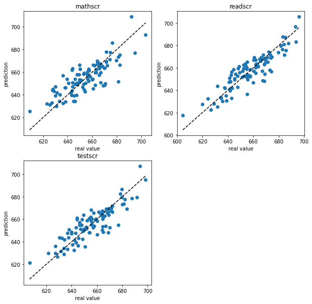
We can see that the predictions seem to follow the real test values rather ok.
Apart from making predictions we can also look at objectives. For example we can evaluate the performance using the Evaluator.
[10]:
performance_1 = causal_structure_1.evaluate_objective(Evaluator, data=data_test,
                                                      inputs=inputs, outputs=outputs,
                                                      metric="r2")
performance_1
[10]:
{'teachers': None,
 'compstu': None,
 'mealpct': None,
 'calwpct': None,
 'str': None,
 'avginc': None,
 'readscr': 0.8020755684153762,
 'enrltot': None,
 'mathscr': 0.6574450121854509,
 'testscr': 0.7577271442716229,
 'computer': None,
 'expnstu': None,
 'elpct': None}
We see that the R2-score for the inputs columns is returned as None. The values for the outputs match with the visual impression of a decent fit.
To judge whether this makes sense we have to know what these columns mean.
[11]:
pydataset.data("Caschool", show_doc=True)
Caschool

PyDataset Documentation (adopted from R Documentation. The displayed examples are in R)

## The California Test Score Data Set

### Description

a cross-section from 1998-1999

_number of observations_ : 420

_observation_ : schools

_country_ : United States

### Usage

    data(Caschool)

### Format

A dataframe containing :

distcod

disctric code

county

county

district

district

grspan

grade span of district

enrltot

total enrollment

teachers

number of teachers

calwpct

percent qualifying for CalWorks

mealpct

percent qualifying for reduced-price lunch

computer

number of computers

testscr

average test score (read.scr+math.scr)/2

compstu

computer per student

expnstu

expenditure per student

str

student teacher ratio

avginc

district average income

elpct

percent of English learners

readscr

average reading score

mathscr

average math score

### Source

California Department of Education http://www.cde.ca.gov.

### References

Stock, James H. and Mark W. Watson (2003) _Introduction to Econometrics_,
Addison-Wesley Educational Publishers,
http://wps.aw.com/aw_stockwatsn_economtrcs_1, chapter 4–7.

### See Also

`Index.Source`, `Index.Economics`, `Index.Econometrics`, `Index.Observations`
We see that in the fully connected model (all inputs influence all outputs) the biggest influences seem to be the total enrollment ‘enrltot’, the amount of teachers ‘teachers’ adn the percentage of students that get subsidized meals ‘mealpct’. The influence of the other tests on ‘testscr’ is zero.
We might now ask the question whether it makes sense that these quantities are the direct main influences or if they are only confounders. If we take a look at the correlations of the inputs, we see that the inputs have significant correlations that can lead to confounding and the explain-away-effect.
[12]:
data_train[inputs].corr().style.background_gradient(cmap='coolwarm', vmin=-1, vmax=1)
[12]:
| teachers | compstu | calwpct | mealpct | str | avginc | enrltot | computer | expnstu | elpct | |
|---|---|---|---|---|---|---|---|---|---|---|
| teachers | 1.000000 | -0.205573 | 0.105457 | 0.142855 | 0.272616 | 0.023591 | 0.997424 | 0.936511 | -0.082112 | 0.357818 |
| compstu | -0.205573 | 1.000000 | -0.171575 | -0.217232 | -0.301937 | 0.183565 | -0.213354 | -0.041737 | 0.274414 | -0.272306 |
| calwpct | 0.105457 | -0.171575 | 1.000000 | 0.735591 | 0.017576 | -0.511519 | 0.099840 | 0.072180 | 0.081346 | 0.350795 |
| mealpct | 0.142855 | -0.217232 | 0.735591 | 1.000000 | 0.155836 | -0.708045 | 0.147787 | 0.076777 | -0.031435 | 0.679559 |
| str | 0.272616 | -0.301937 | 0.017576 | 0.155836 | 1.000000 | -0.222932 | 0.305878 | 0.243671 | -0.590435 | 0.226483 |
| avginc | 0.023591 | 0.183565 | -0.511519 | -0.708045 | -0.222932 | 1.000000 | 0.010920 | 0.076274 | 0.298755 | -0.362238 |
| enrltot | 0.997424 | -0.213354 | 0.099840 | 0.147787 | 0.305878 | 0.010920 | 1.000000 | 0.929746 | -0.100289 | 0.365512 |
| computer | 0.936511 | -0.041737 | 0.072180 | 0.076777 | 0.243671 | 0.076274 | 0.929746 | 1.000000 | -0.061414 | 0.292201 |
| expnstu | -0.082112 | 0.274414 | 0.081346 | -0.031435 | -0.590435 | 0.298755 | -0.100289 | -0.061414 | 1.000000 | -0.049224 |
| elpct | 0.357818 | -0.272306 | 0.350795 | 0.679559 | 0.226483 | -0.362238 | 0.365512 | 0.292201 | -0.049224 | 1.000000 |
We see for example that the total enrollment ‘enrltot’ and the amount of teachers ‘teachers’ are very strongly correlated (also with the amount of computers).
[13]:
data_train.corr().loc[inputs, outputs].T.style.background_gradient(cmap='coolwarm', vmin=-1, vmax=1)
[13]:
| teachers | compstu | calwpct | mealpct | str | avginc | enrltot | computer | expnstu | elpct | |
|---|---|---|---|---|---|---|---|---|---|---|
| testscr | -0.157794 | 0.278550 | -0.628098 | -0.877528 | -0.227190 | 0.734062 | -0.167217 | -0.084573 | 0.150482 | -0.662471 |
| readscr | -0.189992 | 0.285396 | -0.615917 | -0.887392 | -0.252007 | 0.720649 | -0.199871 | -0.117787 | 0.178198 | -0.704534 |
| mathscr | -0.116787 | 0.260359 | -0.617021 | -0.832906 | -0.191503 | 0.720223 | -0.125351 | -0.045295 | 0.114616 | -0.591257 |
Advanced structure#
With the information we have about the data set we can now try to make a more realistic model of the involved columns.
We start with a number of assumptions which result in dependencies.
[14]:
dependencies = []
First of all we see in the data documentation that ‘testscr’ is just the average test score.
[15]:
dependencies += [
    [["mathscr", "readscr"], "testscr"]
]
Assumption 1: We believe the student-teacher-ratio is what actually matters for the test performance. The student teacher ratio of course depends on the number of students and the number of teachers.
[16]:
dependencies += [
    ["str", ["mathscr", "readscr"]],
    [["teachers", "enrltot"], "str"]
]
Assumption 2: We believe the amount of teachers depends on the number of students and the expenses per student.
[17]:
dependencies += [
    [["expnstu", "enrltot"], "teachers"]
]
Assumption 3: The amount of computers per student might indicate the learning possibilities at the school and therefore influence the test results. The amount of computer per student of course is determined by the number of students and the number of computers.
[18]:
dependencies += [
    ["compstu", ["mathscr", "readscr"]],
    [["computer", "enrltot"], "compstu"]
]
Assumption 4: The amount of computers probably depends on the amount of students and the funding per student.
[19]:
dependencies += [
    [["expnstu", "enrltot"], "computer"]
]
Assumption 5: We assume poorer students achieve worse test results on average. In the data we have the percent qualifying for reduced-price lunch ‘mealpct’, the percent qualifying for CalWorks ‘calwpct’ and the average income in the school district ‘avginc’. Since the latter is a bit indirect we assume ‘mealpct’ and ‘calwpct’ are direct influences on the test results while both of them are influenced by ‘avginc’.
[20]:
dependencies += [
    [["mealpct", "calwpct"], ["mathscr", "readscr"]],
    ["avginc", ["mealpct", "calwpct"]]
]
Assumption 6: We assume that being a non-native speaker influences the test results directly as well as the economic situation of the student. The percent of English learners is ‘elpct’.
[21]:
dependencies += [
    ["elpct", ["mathscr", "readscr"]],
    ["elpct", ["mealpct", "calwpct"]]
]
Now we put in these assumptions into a causal structure.
[22]:
causal_structure_2 = CausalStructure(dependencies)
and train it
[23]:
causal_structure_2.train(data_train, method="MGVI")
Let us have a look at the performance on the test data.
[24]:
test_data_inputs = data_test[inputs]
test_data_predictions_2 = causal_structure_2.predict(test_data_inputs)
First visually…
[25]:
import pylab as pl
pl.figure(figsize=(10,10))
for i, col in [(1, "mathscr"), (2, "readscr"), (3, "testscr")]:
    ax = pl.subplot(2,2,i)
    ax.scatter(data_test[col], test_data_predictions_2[col])
    minval, maxval = data_test[col].min(), data_test[col].max()
    ax.plot([minval, maxval], [minval, maxval], ls="--", c="k")
    ax.set_xlabel("real value")
    ax.set_ylabel("prediction")
    ax.set_title(col)
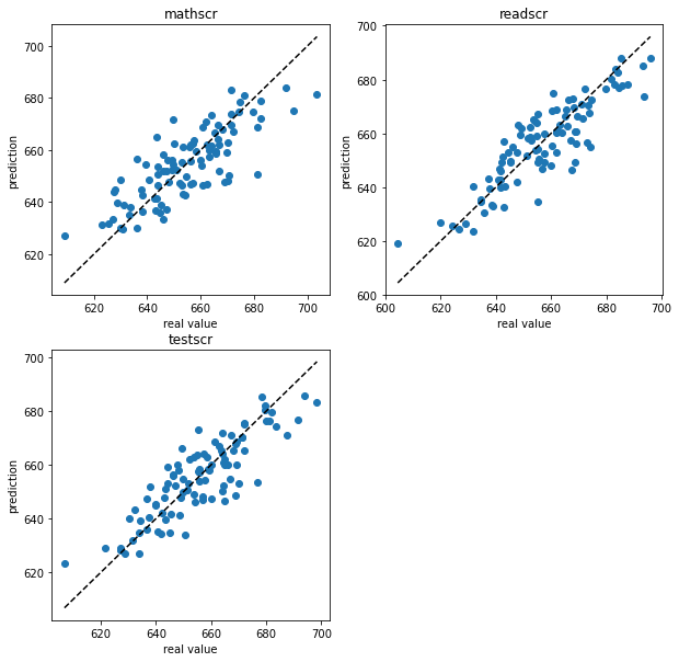
and by the R2 score.
[26]:
performance_2 = causal_structure_2.evaluate_objective(Evaluator, data=data_test,
                                                      inputs=inputs, outputs=outputs,
                                                      metric="r2")
[27]:
display("performance of simple model:")
display({
    key: value for key, value in performance_1.items() if key in outputs
})
display("performance of structured model:")
display({
    key: value for key, value in performance_2.items() if key in outputs
})
'performance of simple model:'
{'readscr': 0.8020755684153762,
 'mathscr': 0.6574450121854509,
 'testscr': 0.7577271442716229}
'performance of structured model:'
{'readscr': 0.7736833098673347,
 'testscr': 0.733377201980135,
 'mathscr': 0.6371819769563171}
We can see that the R2 scores are actually slightly worse than for the simple causal structure, which only had inputs and outputs. Maybe some of our assumptions were incomplete or even wrong.
So what have we gained if the prediction performance is not better? We can see that once we start comparing predicions on partial data.
Comparing the performance of the simple and the advanced structure.#
As we established the performance when predicting the outputs based on all inputs is the same in both models. When all input data are available and the training set and the test set are split randomly it does not matter that much whether the learned behavior is based on real causality or confounders.
However, if we make predictions from incomplete data, this changes.
Example 1: predicting based on subsidized meals and CalWorks#
Let’s try a prediction based on only the amount of subsidized meals and the percentage in the CalWorks program.
[28]:
display("prediction based on simple model:")
display({
    key: value for key, value in
    causal_structure_1.evaluate_objective(Evaluator, data=data_test,
                                          inputs=['calwpct', 'mealpct'], outputs=outputs,
                                          metric="r2").items()
    if key in outputs
})
display("prediction based on structured model:")
display({
    key: value for key, value in
    causal_structure_2.evaluate_objective(Evaluator, data=data_test,
                                          inputs=['calwpct', 'mealpct'], outputs=outputs,
                                          metric="r2").items()
    if key in outputs
})
'prediction based on simple model:'
{'readscr': 0.6342623417400537,
 'mathscr': 0.5509301033970446,
 'testscr': 0.590015453901932}
'prediction based on structured model:'
{'readscr': 0.7078249997685941,
 'testscr': 0.6881614958989846,
 'mathscr': 0.6110603334844447}
We see that in this scenario the structured model outperforms the simple model, but both models still achieve decent scores.
Example 2: predicting based on CalWorks only#
Let’s try a prediction based on only the percentage in the CalWorks program.
[29]:
display("prediction based on simple model:")
display({
    key: value for key, value in
    causal_structure_1.evaluate_objective(Evaluator, data=data_test,
                                          inputs=['calwpct'], outputs=outputs,
                                          metric="r2").items()
    if key in outputs
})
display("prediction based on structured model:")
display({
    key: value for key, value in
    causal_structure_2.evaluate_objective(Evaluator, data=data_test,
                                          inputs=['calwpct'], outputs=outputs,
                                          metric="r2").items()
    if key in outputs
})
'prediction based on simple model:'
{'readscr': -0.033142940725477965,
 'mathscr': 0.11518897669104289,
 'testscr': 0.029182778885538996}
'prediction based on structured model:'
{'readscr': 0.32351923326782916,
 'testscr': 0.3688571477752969,
 'mathscr': 0.37847951309032846}
In this scenario the structured model outperforms the simple model significantly.
Example 3: predicting based on district average income#
Let’s try a prediction based on only the district average income.
[30]:
display("prediction based on simple model:")
display({
    key: value for key, value in
    causal_structure_1.evaluate_objective(Evaluator, data=data_test,
                                          inputs=['avginc'], outputs=outputs,
                                          metric="r2").items()
    if key in outputs
})
display("prediction based on structured model:")
display({
    key: value for key, value in
    causal_structure_2.evaluate_objective(Evaluator, data=data_test,
                                          inputs=['avginc'], outputs=outputs,
                                          metric="r2").items()
    if key in outputs
})
'prediction based on simple model:'
{'readscr': 0.2816587802736583,
 'mathscr': 0.2002535289464773,
 'testscr': 0.2320481281685418}
'prediction based on structured model:'
{'readscr': 0.34039792627046295,
 'testscr': 0.3543316153774535,
 'mathscr': 0.3358698650229551}
In this scenario the structured model outperforms the simple model significantly.
To summarize, a causal structure based on realistic dependency assumptions will not necessarily outperform a black-box model with only inputs and outputs. It is however, more robust when making predicions based on incomplete data.