Estimate probabilities with the Probability Estimator#
The ProbabilityEstimator is an objective class in Halerium, with which one can estimate the probability of certain events.
Ingredients#
To estimate probabilities you only need a graph and data.
Imports#
For the examples below, we need to import the following:
[1]:
# for handling data:
import numpy as np

# for plotting:
import matplotlib.pyplot as plt

# for some Halerium specific functions:
import halerium.core as hal

# for building graphs:
from halerium.core import Graph, Entity, Variable, StaticVariable, show

# for estimating probabilities:
from halerium import ProbabilityEstimator
Basic example#
Let’s create a graph first.
[2]:
g = Graph("g")
with g:
    Variable("z", mean=0, variance=1)
    Variable("x", mean=z, variance=0.1)
    Variable("y", mean=z, variance=0.1)

show(g)
In this graph, both x and y depend on the variable z and follow it fairly closely. The means of x and y are set to z, and the variances of x and y are much smaller than that of z.
Now let’s look at a certain set of data.
[3]:
data = {g.z: [-1, 0, 1., 2., 3.]}
We evaluate the probability that the graph we defined would generate such data points.
[4]:
probability_estimator = ProbabilityEstimator(graph=g, data=data)
We can ask the probability estimator for the probability of any scopetor in the graph.
[5]:
display(probability_estimator(g)) # get the probability of the whole graph
array([-1.41893853, -0.91893853, -1.41893853, -2.91893853, -5.41893853])
We get the logarithmic probability densities for each data point individually. The higher this value, the more likely the event (=data point). We see that the data point with g.z=0 has the highest (least negative) value. It is the most probable event.
Detailed example#
Let’s get some data for g.x and g.y instead of g.z.
[6]:
data = {g.x: [1., -1, -1.],
        g.y: [1., -1,  1.]}
We created three cases here: - one where both x and y are 1, - one where both x and y are -1, and - one where x is -1 and y is 1.
Now we ask the probabilty estimator for the likelihood of these events.
[7]:
probability_estimator = ProbabilityEstimator(g, data)
probability_estimator(g)
[7]:
array([ -1.6222337 , -1.62543181, -11.00601139])
We see that the examples where both x and y are +1 or both are -1 have the same likelihood. But it is very unlikely that one of them is -1 and the other +1.
This reflects that both x and y follow z closely. So they are expexted to be close to each other.
Probabilities of individual variables#
So far we have always asked for the probabilities for the whole graph. We can also ask for probabilities of some sub-structure of the graph, e.g. a specific variable. We just specify it in the call.
For example, we get the probabilities for g.x by:
[8]:
probability_estimator(g.x)
[8]:
array([-1.47250095, -1.49544156, -1.41192295])
or for g.y by:
[9]:
probability_estimator(g.y)
[9]:
array([-1.47250095, -1.49544156, -1.45960488])
We see that the probabilites of the three cases are much closer now. This is because neither g.y = +1 nor g.y = -1 is particularly unlikely. It is only the combination of g.x = -1 and g.y = +1 that was unlikely.
Since g.x and g.y are not causally connected in the sense that one leads to the other you get their independent probabilities if you ask for them seperately.
Missing data#
If some of your data are missing, the probabilities are calculated by marginalizing over the missing values. You can indicate missing value by np.nan.
[10]:
data = {g.x: [-1., np.nan],
        g.y: [ 1.,     1.]}
probability_estimator = ProbabilityEstimator(g, data)
probability_estimator() # the call without any arguments returns a dict of all possible answers.
[10]:
{'g': array([-11.01642622,  -1.45289939]),
 'g/z': array([0., 0.]),
 'g/x': array([-1.4624225,  0.       ]),
 'g/y': array([-1.41741181, -1.45289939])}
We can see that the missing value in g.x yields a logarithmic probability of 0 and the total probability of the graph is equal to the of of g.y.
Background: Logarithmic probability densities#
Note that the class outputs logarithmic probability densities. If we exponentiate these, we get the density.
[11]:
delta_z = 0.01
z_vals = np.arange(-5, 5, delta_z)
log_probs = ProbabilityEstimator(g, {g.z: z_vals})(g)
probs = np.exp(log_probs)
plt.plot(z_vals, np.exp(log_probs));
plt.ylabel("probability density");
plt.xlabel("value of z");
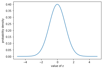
If we integrate that, we get 1.
[12]:
np.sum(probs*delta_z)
[12]:
0.9999994265729888
Background: skewed probability densities#
Graphs are typically constructed out of normal distributions, but the chain of conditional probabilities can produce very different probabilities if non-linear functions are connecting the variables.
Let’s create an example graph.
[13]:
g2 = Graph("g2")
with g2:
    Variable("z", mean=0., variance=1.)
    mu_x = hal.cos(z*3.)
    Variable("x", mean=mu_x, variance=0.01)

delta_x = 0.01
x_vals = np.arange(-1.5, 1.5, delta_x)

log_probs = ProbabilityEstimator(g2, {g2.x: x_vals}, n_samples=10000)(g2)

plt.plot(x_vals, np.exp(log_probs));
plt.xlabel("value of x");
plt.ylabel("probability density");
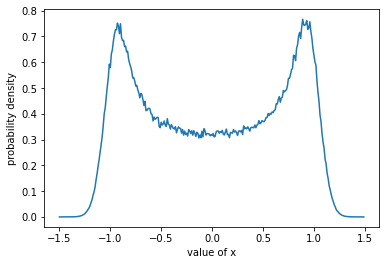
This probability density is clearly not a normal distribution, but it still integrates to 1.
[14]:
np.sum(np.exp(log_probs) * delta_x)
[14]:
0.9984480589771683
[ ]: