Simple training with the Trainer

In Halerium, a model with data for some of its variables usually needs to be “solved” before it can be employed to compute statistical properties consistent with the provided data. This solving step may also be referred to as “fitting the model to the data” (which is roughly what happens under the hood) or (in particular in the context of machine learning) as “training”.

The simplest way to train a model is to use the Trainer class.

The result of the training is the posterior graph representing the trained model. This graph can be used to compute predictions from the trained model, see Outlook, and Predictor.

Imports

We need to import the following packages, classes, and functions.

# for handling data:
import numpy as np

# for plotting
import matplotlib.pyplot as plt

# for graphs:
from halerium.core import Graph, Variable, StaticVariable, show

# for training models
from halerium.core.model import Trainer

# for predictions
from halerium import Predictor

The graph and data

For training models, we need a graph representing the prior statistical properties and connections between variables, and data for some of those variables.

Let us define a simple graph.

graph = Graph("graph")
with graph:
    x = Variable("x", shape=(), mean=0, variance=1**2)
    a = StaticVariable("a", shape=(), mean=1, variance=5**2)
    b = StaticVariable("b", shape=(), mean=0, variance=5**2)
    y = Variable("y", shape=(), mean=a * x + b, variance=1**2)

show(graph)

Now we create some data for training.

true_slope = 2
true_intercept = 1.5

x_train_data = np.linspace(-10, 10, 40)
y_train_data = true_slope * x_train_data + true_intercept + np.random.normal(size=x_train_data.shape)

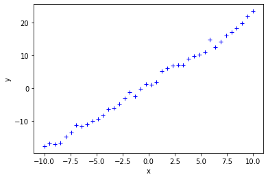
We can plot the training data to get a visual impression.

plt.plot(x_train_data, y_train_data, '+b');
plt.xlabel('x');
plt.ylabel('y');

A Trainer expects the training data in the form of a dictionary with variables in the graph as keys and the data for these variables as values.

train_data = {graph.x: x_train_data, graph.y: y_train_data}

Training with trainer

A Trainer is instantiated with the untrained graph and the training data.

trainer = Trainer(graph=graph,
                  data=train_data)

The instance can then be called to obtain a trained graph.

trained_graph = trainer()

Outlook - Computing predictions

Predictions can be computed using a Predictor (predictor.ipynp) with the trained graph and prediction input data provided upon initialization.

Let’s create some input data for the predictions.

x_prediction_data = np.linspace(-10, 10, 21)
prediction_input_data = {graph.x: x_prediction_data}

Then we create a Predictor instance.

predictor = Predictor(graph=trained_graph,
                      data=prediction_input_data,
                      method="MAP")

We call the predictor with the variable for which we want to have predictions, i.e. graph.y in our case.

y_prediction_data = predictor(graph.y)

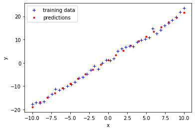
We can plot these predictions on top of the training data.

plt.plot(x_train_data, y_train_data, '+b');
plt.plot(x_prediction_data, y_prediction_data, '.r');
plt.xlabel('x');
plt.ylabel('y');
plt.legend(['training data', 'predictions']);