Training with missing data#
Let us load a data set and have a look
[2]:
import numpy as np
import pandas as pd

x_train = pd.read_csv("training_data_input.csv")
y_train = pd.read_csv("training_data_output.csv")

display(pd.concat([x_train, y_train], axis=1))
| feature_0 | feature_1 | feature_2 | feature_3 | target_0 | target_1 | target_2 | target_3 | |
|---|---|---|---|---|---|---|---|---|
| 0 | 0.472986 | NaN | 0.242439 | -1.700736 | 6.465163 | 1.247767 | 1.562335 | 0.563148 |
| 1 | 0.753143 | -1.534721 | NaN | -0.120228 | NaN | 1.461133 | 1.682604 | -1.078739 |
| 2 | -0.806982 | 2.871819 | NaN | 0.472457 | -2.545614 | NaN | -3.310312 | 0.749930 |
| 3 | NaN | NaN | 1.342356 | -0.122150 | NaN | 1.049569 | 0.504198 | NaN |
| 4 | 1.012515 | -0.913869 | -1.029530 | 1.209796 | NaN | NaN | 1.132657 | -0.651620 |
| ... | ... | ... | ... | ... | ... | ... | ... | ... |
| 95 | 0.078516 | -0.837245 | 1.094795 | NaN | 3.867749 | 1.255217 | 0.865133 | NaN |
| 96 | 0.959965 | -1.167800 | -0.334090 | 0.827424 | 0.544013 | 2.263673 | NaN | -0.057245 |
| 97 | 0.865017 | -0.855405 | 0.071817 | -1.125955 | 5.417294 | 1.349000 | 1.600092 | 0.322496 |
| 98 | -0.206309 | 0.421580 | NaN | 1.481052 | -3.566368 | 1.444973 | -0.434093 | -1.330253 |
| 99 | 0.495926 | NaN | -0.565377 | -0.131805 | 1.555337 | 1.582580 | 0.622529 | 0.949257 |
100 rows × 8 columns
We can see that we have a data set with 4 features and 4 targets. There seem to be lots of missing entries in both the features and the targets.
[3]:
print("missing entries in input data:", "{}%".format(int(np.round(x_train.isna().mean().mean()*100))))
print("missing entries in output data:", "{}%".format(int(np.round(y_train.isna().mean().mean()*100))))
missing entries in input data: 28%
missing entries in output data: 30%
We want to train a linear regression. What can we do about the missing entries?#
Method 1: Mean imputation#
Fill all the missing entries with the mean value of their respective column
[4]:
x_train_imputed = x_train.fillna(value=x_train.mean())
y_train_imputed = y_train.fillna(value=y_train.mean())

display(pd.concat([x_train_imputed, y_train_imputed], axis=1))
| feature_0 | feature_1 | feature_2 | feature_3 | target_0 | target_1 | target_2 | target_3 | |
|---|---|---|---|---|---|---|---|---|
| 0 | 0.472986 | -0.071868 | 0.242439 | -1.700736 | 6.465163 | 1.247767 | 1.562335 | 0.563148 |
| 1 | 0.753143 | -1.534721 | -0.183861 | -0.120228 | 1.655926 | 1.461133 | 1.682604 | -1.078739 |
| 2 | -0.806982 | 2.871819 | -0.183861 | 0.472457 | -2.545614 | 1.605148 | -3.310312 | 0.749930 |
| 3 | 0.064623 | -0.071868 | 1.342356 | -0.122150 | 1.655926 | 1.049569 | 0.504198 | -0.312009 |
| 4 | 1.012515 | -0.913869 | -1.029530 | 1.209796 | 1.655926 | 1.605148 | 1.132657 | -0.651620 |
| ... | ... | ... | ... | ... | ... | ... | ... | ... |
| 95 | 0.078516 | -0.837245 | 1.094795 | -0.093939 | 3.867749 | 1.255217 | 0.865133 | -0.312009 |
| 96 | 0.959965 | -1.167800 | -0.334090 | 0.827424 | 0.544013 | 2.263673 | 0.136459 | -0.057245 |
| 97 | 0.865017 | -0.855405 | 0.071817 | -1.125955 | 5.417294 | 1.349000 | 1.600092 | 0.322496 |
| 98 | -0.206309 | 0.421580 | -0.183861 | 1.481052 | -3.566368 | 1.444973 | -0.434093 | -1.330253 |
| 99 | 0.495926 | -0.071868 | -0.565377 | -0.131805 | 1.555337 | 1.582580 | 0.622529 | 0.949257 |
100 rows × 8 columns
and train a regressor with the imputed data
[5]:
from sklearn.linear_model import LinearRegression
imputed_linear_regression = LinearRegression()
imputed_linear_regression.fit(x_train_imputed, y_train_imputed)
[5]:
LinearRegression()
Method 2: Deletion#
Remove all examples which are missing entries
[6]:
joint_dropped = pd.concat([x_train, y_train], axis=1).dropna(how="any")
x_train_dropped = joint_dropped[x_train.columns]
y_train_dropped = joint_dropped[y_train.columns]

display(pd.concat([x_train_dropped, y_train_dropped], axis=1))
| feature_0 | feature_1 | feature_2 | feature_3 | target_0 | target_1 | target_2 | target_3 | |
|---|---|---|---|---|---|---|---|---|
| 50 | 0.507523 | -0.618371 | 0.790793 | -0.834405 | 3.230641 | 0.885857 | 0.816932 | -0.239825 |
| 54 | -0.809670 | 0.500495 | -0.193510 | -0.664203 | 0.784997 | 1.141402 | -1.039911 | -0.013783 |
| 67 | -1.556314 | -0.693315 | 1.624609 | -0.120666 | -2.247848 | 0.721211 | -0.982030 | -4.287106 |
| 68 | -2.348582 | 0.167257 | 1.699965 | 1.168899 | -7.552532 | 0.995456 | -3.366157 | -5.583932 |
| 70 | -0.488821 | 1.632122 | -0.401225 | 1.009360 | -3.450892 | 1.750701 | -2.670395 | -0.953182 |
| 92 | -1.160888 | -0.579329 | 0.279841 | -0.409602 | 0.251455 | 1.572128 | -0.305981 | -1.609754 |
| 97 | 0.865017 | -0.855405 | 0.071817 | -1.125955 | 5.417294 | 1.349000 | 1.600092 | 0.322496 |
and train a regressor with the remaining data
[7]:
dropped_linear_regression = LinearRegression()
dropped_linear_regression.fit(x_train_dropped, y_train_dropped)
[7]:
LinearRegression()
Method 3: Bayesian model#
A Bayesian model can just treat the missing entries as unknowns
[8]:
import halerium.core as hal
from halerium.core.regression import connect_via_regression

g = hal.Graph("g")
with g:
    x = hal.Variable("x", shape=(4,), mean=0, variance=1)
    y = hal.Variable("y", shape=(4,), variance=0.1)
    connect_via_regression("reg", inputs=[x], outputs=[y], order=1)

# run this to show the graph in the online platform
# hal.show(g)

bayesian_train_model = hal.get_posterior_model(g, data={g.x: x_train, g.y: y_train}, method="MAP")
bayesian_post_graph = bayesian_train_model.get_posterior_graph()
The Bayesian model will actually calculate an estimate for each missing entry (or rather a probability distribution)
[9]:
x_train_bayesian_imputed = bayesian_train_model.get_means(g.x)
x_train_bayesian_imputed = pd.DataFrame(data=x_train_bayesian_imputed, columns=x_train.columns)

from plots import display_side_by_side
display_side_by_side(x_train, x_train_bayesian_imputed)
| feature_0 | feature_1 | feature_2 | feature_3 | |
|---|---|---|---|---|
| 0 | 0.472986 | NaN | 0.242439 | -1.700736 |
| 1 | 0.753143 | -1.534721 | NaN | -0.120228 |
| 2 | -0.806982 | 2.871819 | NaN | 0.472457 |
| 3 | NaN | NaN | 1.342356 | -0.122150 |
| 4 | 1.012515 | -0.913869 | -1.029530 | 1.209796 |
| 5 | 0.501872 | 0.138846 | 0.640761 | NaN |
| 6 | -1.154360 | NaN | -1.681757 | -1.788094 |
| 7 | -2.218535 | -0.647431 | NaN | -0.039209 |
| 8 | NaN | NaN | -0.253904 | 0.073252 |
| 9 | -0.997204 | -0.713856 | NaN | -0.677945 |
| 10 | -0.571881 | -0.105862 | NaN | 0.318665 |
| 11 | -0.337595 | NaN | -0.114920 | 2.241818 |
| 12 | NaN | 0.535136 | 0.232490 | 0.867612 |
| 13 | -1.148213 | NaN | 1.000943 | NaN |
| 14 | NaN | NaN | 0.050523 | NaN |
| 15 | 0.943575 | 0.357644 | -0.083449 | 0.677806 |
| 16 | NaN | 0.222719 | -1.528985 | 1.029211 |
| 17 | -1.166259 | -1.009562 | -0.105268 | 0.512022 |
| 18 | 1.407728 | NaN | 1.471234 | NaN |
| 19 | -0.461395 | NaN | -0.571817 | -0.603299 |
| 20 | -1.339389 | -1.689653 | NaN | 0.257773 |
| 21 | 1.828821 | -1.001002 | -2.091691 | 0.146560 |
| 22 | -0.466351 | NaN | NaN | -1.259224 |
| 23 | NaN | 0.802630 | 0.272391 | -0.969176 |
| 24 | 0.871968 | -1.446359 | NaN | 0.197921 |
| 25 | -1.365640 | NaN | 0.015935 | -0.080043 |
| 26 | -0.250803 | -0.565143 | NaN | -0.782282 |
| 27 | 3.041686 | -0.626081 | NaN | -0.587336 |
| 28 | NaN | 1.232045 | 0.450889 | -0.641410 |
| 29 | NaN | 0.965746 | -1.284003 | -1.274572 |
| 30 | 1.522842 | 1.461882 | 0.037656 | -0.246197 |
| 31 | NaN | NaN | NaN | -1.513087 |
| 32 | NaN | 0.249203 | NaN | NaN |
| 33 | NaN | 1.689292 | 0.177750 | 0.032006 |
| 34 | 1.933216 | -1.062095 | -0.732629 | 0.842741 |
| 35 | 1.076740 | NaN | -2.619493 | 0.739046 |
| 36 | 0.667501 | NaN | NaN | 1.407948 |
| 37 | 0.051149 | -0.935975 | -1.839109 | NaN |
| 38 | NaN | -0.561885 | -1.132469 | 0.274291 |
| 39 | 0.735912 | 0.434319 | -1.120041 | 0.889095 |
| 40 | NaN | -2.488004 | 0.595909 | -2.035862 |
| 41 | NaN | 1.057642 | 0.652769 | NaN |
| 42 | -0.883462 | 0.345692 | NaN | 0.410710 |
| 43 | NaN | 0.734148 | -0.125496 | NaN |
| 44 | 0.202231 | NaN | -1.421277 | -1.163588 |
| 45 | NaN | 0.050022 | 0.765430 | -0.028515 |
| 46 | -1.205646 | NaN | 0.566844 | NaN |
| 47 | -0.940359 | 0.283607 | -0.390320 | -2.154124 |
| 48 | NaN | -0.566221 | -0.517709 | NaN |
| 49 | -0.603695 | NaN | -0.959012 | -1.595297 |
| 50 | 0.507523 | -0.618371 | 0.790793 | -0.834405 |
| 51 | 1.309470 | -1.238742 | NaN | 0.696147 |
| 52 | 1.778984 | -0.796317 | NaN | NaN |
| 53 | 0.789916 | NaN | -2.184060 | -1.567268 |
| 54 | -0.809670 | 0.500495 | -0.193510 | -0.664203 |
| 55 | NaN | -1.658425 | NaN | NaN |
| 56 | 1.269859 | 0.150519 | NaN | NaN |
| 57 | NaN | 0.164989 | NaN | -0.115399 |
| 58 | NaN | NaN | 0.475514 | 2.639046 |
| 59 | 0.691108 | 1.111236 | -0.257684 | -1.195951 |
| 60 | NaN | -1.163467 | -3.015915 | NaN |
| 61 | 0.331393 | -1.072815 | NaN | -0.085521 |
| 62 | -0.476624 | -0.963715 | 1.153983 | -0.444866 |
| 63 | NaN | -0.474993 | -0.791428 | -1.693119 |
| 64 | -0.741163 | NaN | NaN | NaN |
| 65 | NaN | NaN | -0.818418 | -0.177300 |
| 66 | 0.032502 | NaN | NaN | 0.210377 |
| 67 | -1.556314 | -0.693315 | 1.624609 | -0.120666 |
| 68 | -2.348582 | 0.167257 | 1.699965 | 1.168899 |
| 69 | 0.055338 | 0.217881 | NaN | -0.158261 |
| 70 | -0.488821 | 1.632122 | -0.401225 | 1.009360 |
| 71 | -1.577518 | -0.788323 | -1.156447 | 0.410545 |
| 72 | -0.633212 | -0.650858 | -0.925059 | 0.143164 |
| 73 | 0.975512 | -0.599755 | 0.607099 | -0.018603 |
| 74 | -0.621560 | 0.346610 | 1.337491 | NaN |
| 75 | 0.695248 | NaN | NaN | 0.763436 |
| 76 | 0.976937 | 0.517606 | 0.249171 | 1.304453 |
| 77 | 1.116544 | NaN | 0.662984 | -0.904909 |
| 78 | -0.158939 | NaN | -0.043852 | -0.666356 |
| 79 | NaN | NaN | NaN | -1.300151 |
| 80 | -0.511364 | -0.692839 | NaN | 1.682377 |
| 81 | NaN | 0.200962 | 0.376479 | -0.193338 |
| 82 | -0.536373 | NaN | -0.405771 | NaN |
| 83 | NaN | NaN | 0.331393 | NaN |
| 84 | 0.980989 | NaN | NaN | NaN |
| 85 | -0.077496 | 0.410431 | 0.275277 | 0.525207 |
| 86 | NaN | 2.193451 | -0.159283 | NaN |
| 87 | 0.168298 | 1.370530 | -0.728801 | NaN |
| 88 | 1.229295 | 0.779550 | 0.215736 | NaN |
| 89 | 1.290819 | 0.455251 | -0.571328 | -0.465401 |
| 90 | -0.632571 | 1.413624 | -0.167273 | NaN |
| 91 | -0.579659 | 1.121277 | 0.619558 | NaN |
| 92 | -1.160888 | -0.579329 | 0.279841 | -0.409602 |
| 93 | NaN | 0.020903 | -0.576144 | -1.103720 |
| 94 | NaN | -0.939964 | -0.722252 | 0.251525 |
| 95 | 0.078516 | -0.837245 | 1.094795 | NaN |
| 96 | 0.959965 | -1.167800 | -0.334090 | 0.827424 |
| 97 | 0.865017 | -0.855405 | 0.071817 | -1.125955 |
| 98 | -0.206309 | 0.421580 | NaN | 1.481052 |
| 99 | 0.495926 | NaN | -0.565377 | -0.131805 |
| feature_0 | feature_1 | feature_2 | feature_3 | |
|---|---|---|---|---|
| 0 | 0.472986 | -0.759207 | 0.242439 | -1.700736 |
| 1 | 0.753143 | -1.534721 | 0.360400 | -0.120228 |
| 2 | -0.806982 | 2.871819 | -0.901917 | 0.472457 |
| 3 | 0.533772 | -1.179473 | 1.342356 | -0.122150 |
| 4 | 1.012515 | -0.913869 | -1.029530 | 1.209796 |
| 5 | 0.501872 | 0.138846 | 0.640761 | 0.462867 |
| 6 | -1.154360 | 0.000016 | -1.681757 | -1.788094 |
| 7 | -2.218535 | -0.647431 | -0.350765 | -0.039209 |
| 8 | 0.180386 | -0.439187 | -0.253904 | 0.073252 |
| 9 | -0.997204 | -0.713856 | 0.246540 | -0.677945 |
| 10 | -0.571881 | -0.105862 | 1.447496 | 0.318665 |
| 11 | -0.337595 | -1.091010 | -0.114920 | 2.241818 |
| 12 | -2.736205 | 0.535136 | 0.232490 | 0.867612 |
| 13 | -1.148213 | 1.240510 | 1.000943 | 0.583911 |
| 14 | -0.133397 | -0.819823 | 0.050523 | -0.434769 |
| 15 | 0.943575 | 0.357644 | -0.083449 | 0.677806 |
| 16 | 0.394197 | 0.222719 | -1.528985 | 1.029211 |
| 17 | -1.166259 | -1.009562 | -0.105268 | 0.512022 |
| 18 | 1.407728 | -1.550861 | 1.471234 | 1.608291 |
| 19 | -0.461395 | -0.631948 | -0.571817 | -0.603299 |
| 20 | -1.339389 | -1.689653 | -0.118997 | 0.257773 |
| 21 | 1.828821 | -1.001002 | -2.091691 | 0.146560 |
| 22 | -0.466351 | 0.208242 | 0.408953 | -1.259224 |
| 23 | -0.410407 | 0.802630 | 0.272391 | -0.969176 |
| 24 | 0.871968 | -1.446359 | -0.259302 | 0.197921 |
| 25 | -1.365640 | -1.612685 | 0.015935 | -0.080043 |
| 26 | -0.250803 | -0.565143 | -0.917229 | -0.782282 |
| 27 | 3.041686 | -0.626081 | 1.193158 | -0.587336 |
| 28 | 1.073791 | 1.232045 | 0.450889 | -0.641410 |
| 29 | -1.003597 | 0.965746 | -1.284003 | -1.274572 |
| 30 | 1.522842 | 1.461882 | 0.037656 | -0.246197 |
| 31 | -0.706564 | 0.145486 | -0.472127 | -1.513087 |
| 32 | 0.418605 | 0.249203 | -1.133117 | -0.512646 |
| 33 | 0.436980 | 1.689292 | 0.177750 | 0.032006 |
| 34 | 1.933216 | -1.062095 | -0.732629 | 0.842741 |
| 35 | 1.076740 | 0.069814 | -2.619493 | 0.739046 |
| 36 | 0.667501 | -0.219459 | 0.635413 | 1.407948 |
| 37 | 0.051149 | -0.935975 | -1.839109 | -0.060533 |
| 38 | -0.575251 | -0.561885 | -1.132469 | 0.274291 |
| 39 | 0.735912 | 0.434319 | -1.120041 | 0.889095 |
| 40 | 0.044935 | -2.488004 | 0.595909 | -2.035862 |
| 41 | -0.001871 | 1.057642 | 0.652769 | 0.003109 |
| 42 | -0.883462 | 0.345692 | -1.679739 | 0.410710 |
| 43 | 0.109791 | 0.734148 | -0.125496 | -0.897293 |
| 44 | 0.202231 | -0.035420 | -1.421277 | -1.163588 |
| 45 | -1.291495 | 0.050022 | 0.765430 | -0.028515 |
| 46 | -1.205646 | -0.207500 | 0.566844 | 0.835726 |
| 47 | -0.940359 | 0.283607 | -0.390320 | -2.154124 |
| 48 | -0.443188 | -0.566221 | -0.517709 | 0.358158 |
| 49 | -0.603695 | 0.184274 | -0.959012 | -1.595297 |
| 50 | 0.507523 | -0.618371 | 0.790793 | -0.834405 |
| 51 | 1.309470 | -1.238742 | -1.157520 | 0.696147 |
| 52 | 1.778984 | -0.796317 | 0.926392 | 1.833046 |
| 53 | 0.789916 | -0.119241 | -2.184060 | -1.567268 |
| 54 | -0.809670 | 0.500495 | -0.193510 | -0.664203 |
| 55 | 0.654011 | -1.658425 | 0.240789 | -0.615273 |
| 56 | 1.269859 | 0.150519 | -1.137418 | -0.680453 |
| 57 | -1.376112 | 0.164989 | -1.365167 | -0.115399 |
| 58 | 0.894641 | 0.094943 | 0.475514 | 2.639046 |
| 59 | 0.691108 | 1.111236 | -0.257684 | -1.195951 |
| 60 | -0.217195 | -1.163467 | -3.015915 | 0.357342 |
| 61 | 0.331393 | -1.072815 | 1.607594 | -0.085521 |
| 62 | -0.476624 | -0.963715 | 1.153983 | -0.444866 |
| 63 | -0.220168 | -0.474993 | -0.791428 | -1.693119 |
| 64 | -0.741163 | -0.666493 | 0.601783 | -1.320586 |
| 65 | 0.498025 | -0.692433 | -0.818418 | -0.177300 |
| 66 | 0.032502 | -0.380547 | 0.508512 | 0.210377 |
| 67 | -1.556314 | -0.693315 | 1.624609 | -0.120666 |
| 68 | -2.348582 | 0.167257 | 1.699965 | 1.168899 |
| 69 | 0.055338 | 0.217881 | 0.491295 | -0.158261 |
| 70 | -0.488821 | 1.632122 | -0.401225 | 1.009360 |
| 71 | -1.577518 | -0.788323 | -1.156447 | 0.410545 |
| 72 | -0.633212 | -0.650858 | -0.925059 | 0.143164 |
| 73 | 0.975512 | -0.599755 | 0.607099 | -0.018603 |
| 74 | -0.621560 | 0.346610 | 1.337491 | -2.588218 |
| 75 | 0.695248 | 0.598883 | 0.739468 | 0.763436 |
| 76 | 0.976937 | 0.517606 | 0.249171 | 1.304453 |
| 77 | 1.116544 | 0.133607 | 0.662984 | -0.904909 |
| 78 | -0.158939 | 0.230231 | -0.043852 | -0.666356 |
| 79 | 1.125959 | 0.713062 | 0.539098 | -1.300151 |
| 80 | -0.511364 | -0.692839 | -0.747252 | 1.682377 |
| 81 | 2.397169 | 0.200962 | 0.376479 | -0.193338 |
| 82 | -0.536373 | 1.193916 | -0.405771 | -1.085892 |
| 83 | 0.728069 | -0.042654 | 0.331393 | 0.364764 |
| 84 | 0.980989 | 0.735467 | 0.519223 | 0.578556 |
| 85 | -0.077496 | 0.410431 | 0.275277 | 0.525207 |
| 86 | -0.014028 | 2.193451 | -0.159283 | 0.273037 |
| 87 | 0.168298 | 1.370530 | -0.728801 | -1.226624 |
| 88 | 1.229295 | 0.779550 | 0.215736 | -0.646722 |
| 89 | 1.290819 | 0.455251 | -0.571328 | -0.465401 |
| 90 | -0.632571 | 1.413624 | -0.167273 | -1.041896 |
| 91 | -0.579659 | 1.121277 | 0.619558 | -0.399106 |
| 92 | -1.160888 | -0.579329 | 0.279841 | -0.409602 |
| 93 | -0.364879 | 0.020903 | -0.576144 | -1.103720 |
| 94 | -0.851016 | -0.939964 | -0.722252 | 0.251525 |
| 95 | 0.078516 | -0.837245 | 1.094795 | -1.177459 |
| 96 | 0.959965 | -1.167800 | -0.334090 | 0.827424 |
| 97 | 0.865017 | -0.855405 | 0.071817 | -1.125955 |
| 98 | -0.206309 | 0.421580 | -0.704793 | 1.481052 |
| 99 | 0.495926 | 0.324680 | -0.565377 | -0.131805 |
Compare the performance on test data#
[10]:
x_test = pd.read_csv("testing_data_input.csv").values
y_test = pd.read_csv("testing_data_output.csv").values

imputed_prediction = imputed_linear_regression.predict(x_test)

dropped_prediction = dropped_linear_regression.predict(x_test)

bayesian_prediction_model = hal.get_generative_model(bayesian_post_graph, data={g.x: x_test})
bayesian_prediction = bayesian_prediction_model.get_means(g.y)
[11]:
import pylab as pl

pl.figure(figsize=(12, 12))

dark_erium_green = '#00b34a'
erium_blue = '#002a43'

ax = pl.subplot(2,2,1)
ax.set_aspect("equal")
ax.scatter(y_test[:,0], imputed_prediction[:,0], color='#00b34a')
ax.plot([np.min(y_test[:,0]),np.max(y_test[:,0])], [np.min(y_test[:,0]),np.max(y_test[:,0])], ls=":", color="k")
ax.set_xlabel("real output value")
ax.set_ylabel("predicted output value")
ax.set_title("training with imputed data")

ax = pl.subplot(2,2,2)
ax.set_aspect("equal")
ax.scatter(y_test[:,0], dropped_prediction[:,0], color='#00b34a')
ax.plot([np.min(y_test[:,0]),np.max(y_test[:,0])], [np.min(y_test[:,0]),np.max(y_test[:,0])], ls=":", color="k")
ax.set_xlabel("real output value")
ax.set_ylabel("predicted output value")
ax.set_title("training with missing rows dropped")

ax = pl.subplot(2,1,2)
ax.set_aspect("equal")
ax.scatter(y_test[:,0], bayesian_prediction[:,0], color='#00b34a')
ax.plot([np.min(y_test[:,0]),np.max(y_test[:,0])], [np.min(y_test[:,0]),np.max(y_test[:,0])], ls=":", color="k")
ax.set_xlabel("real output value")
ax.set_ylabel("predicted output value")
ax.set_title("Bayesian model")
[11]:
Text(0.5, 1.0, 'Bayesian model')
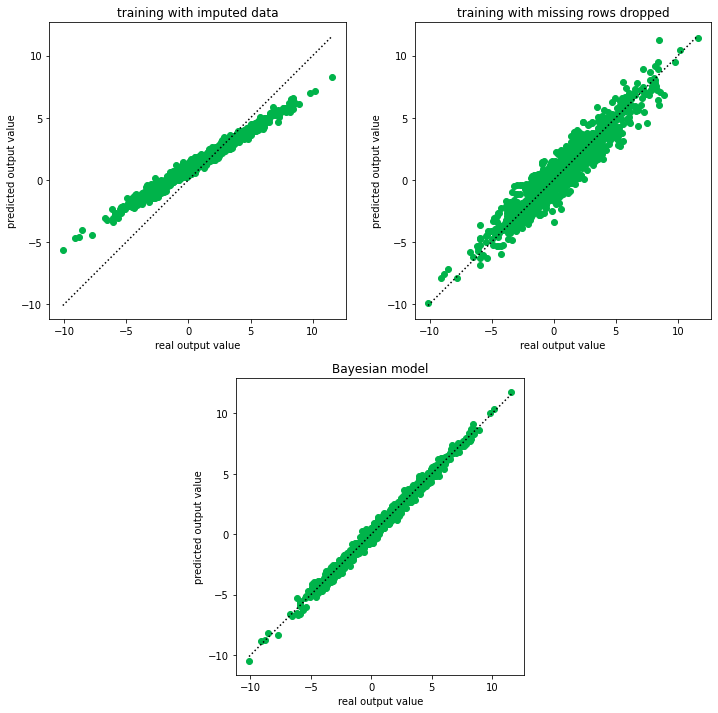
As you can see, Bayesian models offer interesting advantages when dealing with missing data. Missing data often occur in industrial environments, e.g. when a sensor output could not be recorded or the output was corrupted.
[ ]: