More on training models

In Halerium, a model with data for some of its variables usually needs to be “solved” before it can be employed to compute statistical properties consistent with the provided data. This solving step may also be referred to as “fitting the model to the data” (which is roughly what happens under the hood) or (in particular in the context of machine learning) as “training”.

Models can be created and trained using the model factory function get_posterior_model, see Training with model factories.

Models can also be created and trained using the halerium.model classes and their methods directly, see Training models directly.

Moreover, models can be trained using The Trainer class, see Trainer.

The result of the training is the posterior graph representing the trained model. This graph can be used to compute predictions from the trained model, see Outlook, and Predictor.

Imports

We need to import the following packages, classes, and functions.

# for handling data:
import numpy as np

# for plotting:
import matplotlib.pyplot as plt

# for graphs:
from halerium.core import Graph, Variable, StaticVariable, show

# for creating models with a factory:
from halerium.core.model import get_posterior_model

# for creating and using models directly:
from halerium.core.model import MAPModel, MAPFisherModel, ForwardModel

The graph and data

For training models, we need a graph representing the prior statistical properties and connections between variables, and data for some of those variables.

Let us define a simple graph.

graph = Graph("graph")
with graph:
    x = Variable("x", shape=(), mean=0, variance=1**2)
    a = StaticVariable("a", shape=(), mean=1, variance=5**2)
    b = StaticVariable("b", shape=(), mean=0, variance=5**2)
    y = Variable("y", shape=(), mean=a * x + b, variance=1**2)


show(graph)

Now we create some data for training.

true_slope = 2
true_intercept = 1.5

x_train_data = np.linspace(-10, 10, 40)
y_train_data = true_slope * x_train_data + true_intercept + np.random.normal(size=x_train_data.shape)

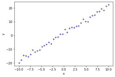
We can plot the training data to get a visual impression.

plt.plot(x_train_data, y_train_data, '+b');
plt.xlabel('x');
plt.ylabel('y');

When using model factories, the training data can be passed as a dictionary specifying the association of the variables in the graph and the data.

train_data = {graph.x: x_train_data, graph.y: y_train_data}

Training with model factories

To create and train a model, one can employ the get_posterior_model function. The data for training can be directly provided as a dictionary.

model = get_posterior_model(graph=graph, data=train_data)

Unless specified otherwise, the model is already solved, and one can directly obtain the posterior graph.

trained_graph = model.get_posterior_graph()

Training models directly

Models can also be created and trained using the Halerium.model classes and their methods directly.

First, we pick a model class suitable for training, e.g. a MAPModel. Then we create a model instance of that class. For that, we have to provide the graph and the data packaged into a data linker.

model = MAPModel(graph=graph,
                 data=train_data)

We can train the model using the solve method.

model.solve()

As a result, the model has adjusted the distribution of the model parameters graph.a and graph.b according to the training data.

a_trained_mean = model.get_means(graph.a)
b_trained_mean = model.get_means(graph.b)

print("trained mean for a:", a_trained_mean)
print("trained mean for b:", b_trained_mean)

trained mean for a: 2.0128642238484
trained mean for b: 1.4387307591662526

We can now obtain a trained graph.

trained_graph = model.get_posterior_graph()

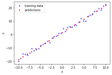
Outlook: Using a trained model for predictions

The trained graph can be used to compute predictions, e.g., for graph.y given new data for graph.x. We create new data for graph.x, a new model with the trained graph and the new data as input data, solve that model, and extract values from the model for graph.y given the new data for graph.x.

x_prediction_data = np.linspace(-10, 10, 21)

prediction_input_data = {graph.x: x_prediction_data}

trained_model = MAPModel(graph=trained_graph,
                         data=prediction_input_data)

trained_model.solve()
y_prediction_data = trained_model.get_means(graph.y)
print("predicted values for y:", y_prediction_data)

predicted values for y: [-18.68991148 -16.67704726 -14.66418303 -12.65131881 -10.63845458
  -8.62559036  -6.61272614  -4.59986191  -2.58699769  -0.57413346
   1.43873076   3.45159498   5.46445921   7.47732343   9.49018765
  11.50305188  13.5159161   15.52878033  17.54164455  19.55450877
  21.567373  ]

plt.plot(x_train_data, y_train_data, '+b');
plt.plot(x_prediction_data, y_prediction_data, '.r');
plt.xlabel('x');
plt.ylabel('y');
plt.legend(['training data', 'predictions']);