Logistic regression

Logistic regression can be used to learn the probability of an event being true or false as a function of one or more features.

Here we present as example a simple ‘linear’ logistic regression.

Imports

We import the following packages, classes, and functions.

# for handling data:
import numpy as np
import pandas as pd

# for plotting:
import matplotlib.pyplot as plt

import halerium.core as hal

# for graphs:
from halerium.core import Graph, Entity, Variable, StaticVariable
from halerium.core.regression import linear_regression, polynomial_regression, connect_via_regression
from halerium.core.distribution import BernoulliDistribution

# for models:
from halerium.core import DataLinker, get_data_linker
from halerium.core.model import MAPModel, ForwardModel, Trainer
from halerium.core.model import get_posterior_model

# for predictions:
from halerium import Predictor

Example data

To create example data, we simply build a forward model of logistic regression:

n_data = 100

x_scatter = 10

with Graph("graph") as graph:

    x = Variable("x", shape=(2,), mean=0, variance=x_scatter**2)
    y = Variable("y",  shape=(), distribution=BernoulliDistribution)

    connect_via_regression(
        name_prefix="parameters",
        inputs=x,
        outputs=y,
        order=1,
    )

slope = graph.parameters_y.location.slope
intercept = graph.parameters_y.location.intercept

model = ForwardModel(graph, data=DataLinker(n_data))
x_data, y_data, slope_data, intercept_data = model.get_example((x, y, slope, intercept))

data = pd.DataFrame()
data["x_1"] = x_data[:,0]
data["x_2"] = x_data[:,1]
data["y"] = y_data

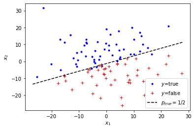
Let’s visualize the generated data:

x_true = x_data[y_data]
x_false = x_data[~y_data]
plt.plot(x_true[:,0], x_true[:,1], '.b')
plt.plot(x_false[:,0], x_false[:,1], '+r')

r = np.linspace((-1,-1), (1, 1)) * 3 * x_scatter / np.linalg.norm(slope_data)
x_r = r * (np.array([[0,1],[-1,0]]) @ slope_data) - intercept_data / np.linalg.norm(slope_data)**2 * slope_data
plt.plot(x_r[:,0], x_r[:,1], '--k');
plt.xlabel("$x_1$");
plt.ylabel("$x_2$");
plt.legend(["$y$=true", "$y$=false", "$p_{true}=1/2$"]);

Logistic regression model

Now let us bulid an train a logistic regression model.

with Graph("graph") as graph:

    x = Variable("x", shape=(2,), mean=0, variance=x_scatter**2)
    y = Variable("y",  shape=(), distribution=BernoulliDistribution)

    connect_via_regression(
        name_prefix="parameters",
        inputs=x,
        outputs=y,
        order=1,
    )

trained_graph = Trainer(graph=graph, data = {graph.x: data[["x_1", "x_2"]], graph.y: data["y"]})()

trained_graph.parameters_y.location.slope.mean

<halerium.Const at 0x24cc2d0a688: name='Const', shape=(2,), global_name='graph/parameters_y/location/slope/Const', dynamic=False>

We can use the trained graph to predict the probability of y=true for a given set of x-values:

prediction_x_data = np.linspace((-10, 0), (10, 0), 11)

predictor = Predictor(graph=trained_graph, data={trained_graph.x: prediction_x_data}, n_samples=1000)
prediction_y_data = predictor(trained_graph.y)

prediction_data = pd.DataFrame()
prediction_data["x_1"] = prediction_x_data[:,0]
prediction_data["x_2"] = prediction_x_data[:,1]
prediction_data["p_y_pred"] = prediction_y_data
display(prediction_data)

	x_1	x_2	p_y_pred
0	-10.0	0.0	0.913
1	-8.0	0.0	0.854
2	-6.0	0.0	0.812
3	-4.0	0.0	0.718
4	-2.0	0.0	0.619
5	0.0	0.0	0.505
6	2.0	0.0	0.396
7	4.0	0.0	0.293
8	6.0	0.0	0.198
9	8.0	0.0	0.150
10	10.0	0.0	0.094

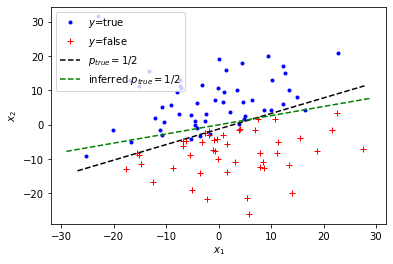
We can also compare the predicted vs. true \(p_{true}=1/2\)-line:

x_true = data[data["y"]][["x_1", "x_2"]]
x_false = data[~data["y"]][["x_1", "x_2"]]

plt.plot(x_true["x_1"], x_true["x_2"], '.b')
plt.plot(x_false["x_1"], x_false["x_2"], '+r')

r = np.linspace((-1,-1), (1, 1)) * 3 * x_scatter / np.linalg.norm(slope_data)
x_r = r * (np.array([[0,1],[-1,0]]) @ slope_data) - intercept_data / np.linalg.norm(slope_data)**2 * slope_data
plt.plot(x_r[:,0], x_r[:,1], '--k');

inferred_slope_data = predictor(trained_graph.parameters_y.location.slope)
inferred_intercept_data =  predictor(trained_graph.parameters_y.location.intercept)

s = np.linspace((-1,-1), (1, 1)) * 3 * x_scatter / np.linalg.norm(inferred_slope_data)
x_s = s * (np.array([[0,1],[-1,0]]) @ inferred_slope_data) - inferred_intercept_data / np.linalg.norm(inferred_slope_data)**2 * inferred_slope_data
plt.plot(x_s[:,0], x_s[:,1], '--g');



plt.xlabel("$x_1$");
plt.ylabel("$x_2$");
plt.legend(["$y$=true", "$y$=false", "$p_{true}=1/2$", "inferred $p_{true}=1/2$"]);